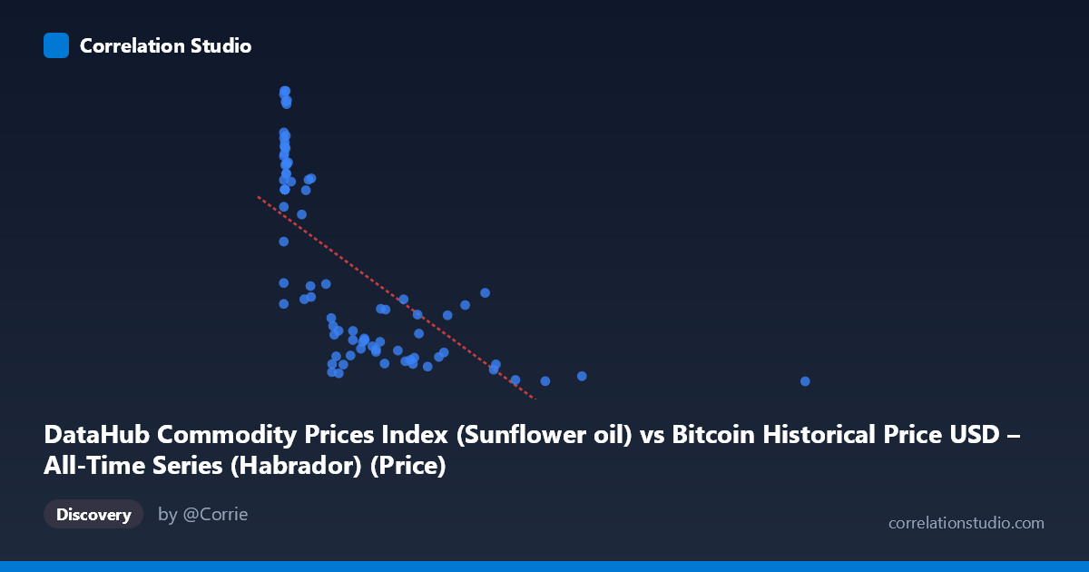
DataHub Commodity Prices Index (Sunflower oil) vs Bitcoin Historical Price USD – All-Time Series (Habrador) (Price)
- Pearson correlation (r)
- -0.6685
- Spearman correlation
- -0.7879
- p-value
- 0
- Sample size (n)
- 83
- 95% confidence interval
- -0.7728 to -0.5291
- Granger causality
- None
- Granger optimal lag
- 10
- Time coverage
- 2010-08-01 to 2017-06-01
AI analysis
Analysis: Sunflower Oil Price Index vs. Bitcoin Historical Price (USD)
1. Relationship Overview
The scatterplot shows a clear inverse relationship between the sunflower oil commodity index (X) and Bitcoin price (Y), though the shape is distinctly non-linear rather than a simple straight-line decline. Data points cluster heavily in the low-X region (below ~300), where Y values span a wide range from roughly 950 to 1700. As X increases beyond ~600, Y values compress into a narrower, lower band (900–1150), and the single extreme outlier at X=2452.18 anchors the far right with Y=936.24, one of the lowest values in the dataset. This pattern resembles a decaying curve (logarithmic or power-law) more than a linear trend.
2. Strength, Direction, and Statistical Confidence
The Pearson correlation of r = -0.6685 indicates a moderately strong negative linear relationship, with r² = 0.447 meaning the linear model explains only about 45% of the variance in Bitcoin price — leaving over half unexplained by X alone. The 95% CI [-0.7728, -0.5291] is reasonably tight and entirely negative, and the p-value (4.99E-12) is highly significant, so we can be confident a real negative association exists in this sample — this is not a chance artifact. However, the note that Spearman's ρ exceeds Pearson's r is important: it suggests the true relationship is monotonic but curved, and a log or polynomial fit would likely capture meaningfully more variance than the 44.7% linear R².
Critically, the Granger causality tests show no significant predictive direction in either direction (X→Y: p=0.51; Y→X: p=0.17) at 10 lags. This means despite the strong contemporaneous correlation, neither series reliably forecasts the other's future movements in a time-series sense. This is a crucial distinction: correlation here reflects concurrent co-movement, not a lead-lag causal mechanism.
3. Notable Patterns and Outliers
Several features stand out: - Dense low-X cluster: The majority of points sit at X < 50, with Y ranging widely (1400–1700), suggesting high Bitcoin price volatility during periods of low/stable sunflower oil pricing — likely corresponding to Bitcoin's early years (2010–2013) before major bull runs. - Mid-range compression: Between X=200–800, Y values tighten into the 950–1150 range, suggesting a more stable, lower Bitcoin valuation regime. - High-leverage outlier: The point at (2452.18, 936.24) is far separated from all other X values and could disproportionately influence the linear regression slope and correlation strength. - Curved decay shape: The overall pattern looks like Y ~ a/X or Y ~ log(X), consistent with the Spearman/Pearson discrepancy noted.
4. Confounding Factors and Caveats
This correlation is almost certainly spurious or indirect rather than causal. Both series are independent economic time series (a commodity price index and Bitcoin price) that happen to span overlapping calendar periods (2010–2017) — a period when Bitcoin underwent enormous secular growth unrelated to sunflower oil markets. Any two long-term trending or highly volatile series can show statistical correlation purely from time-based co-trending (a classic spurious correlation risk in time series analysis). The lack of Granger causality reinforces that these series aren't mechanistically linked — they're likely both correlated with a third factor (time/macroeconomic cycles) rather than with each other directly. Additionally, the small paired sample (n=83) relative to the full population (N=449) means substantial sampling variability could affect the exact correlation estimate, and the single extreme X outlier may be inflating the apparent linear relationship.
5. Suggestions for Further Investigation
- Refit with non-linear models (log-X, power, or polynomial) to test whether R² improves substantially, as hinted by the Spearman/Pearson gap. - Detrend both series (e.g., first-difference or remove long-term trend) before correlating, to check if the relationship persists once shared time-trend is removed — this would test for genuine co-movement vs. spurious trend correlation. - Exclude or separately analyze the extreme outlier (X=2452.18) to assess its influence on regression coefficients and correlation strength. - Investigate an underlying confound, such as USD strength, global risk sentiment, or inflation expectations, which could simultaneously affect both commodity prices and Bitcoin valuations during 2010–2017. - Given no Granger causality, avoid using this relationship for predictive trading models; treat it as a descriptive/historical association only.
X dataset: Bitcoin Historical Price USD – All-Time Series (Habrador)
Y dataset: DataHub Commodity Prices Index
Part of experiment: Bitcoin - Bitcoin Historical Price USD – All-Time Series (Habrador) vs DataHub Commodity Prices Index