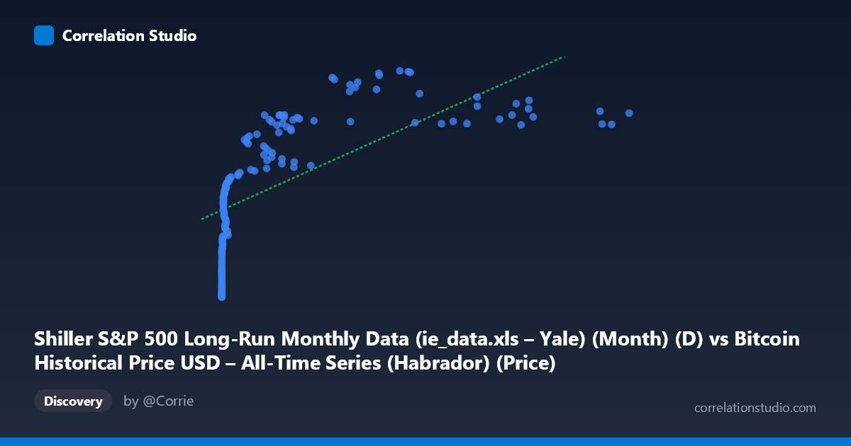
Shiller S&P 500 Long-Run Monthly Data (ie_data.xls – Yale) (Month) (D) vs Bitcoin Historical Price USD – All-Time Series (Habrador) (Price)
- Pearson correlation (r)
- 0.6646
- Spearman correlation
- 0.9478
- p-value
- 0
- Sample size (n)
- 155
- 95% confidence interval
- 0.5663 to 0.7443
- Granger causality
- None
- Granger optimal lag
- 1
- Time coverage
- 2010-08-01 to 2023-06-01
- Recomputed on refreshed data
- 2026-10-10 (r was 0.6646)
AI analysis
Analysis: Bitcoin Price vs. S&P 500 (Shiller Data)
1. Relationship Overview
The scatterplot shows a positive but non-linear association between Bitcoin's price and the S&P 500 series. At very low Bitcoin prices (near $0–$15, corresponding to Bitcoin's earliest years, 2010–2011), Y values cluster tightly in the low 20s–30s range. As Bitcoin's price climbs into the thousands and tens of thousands of dollars, Y rises and plateaus in the 55–68 range, with considerable scatter at high X values. The relationship resembles a logarithmic or saturating curve rather than a straight line — rapid Y growth at low X, flattening as X increases.
2. Strength, Direction, and Uncertainty
The Pearson correlation (r = 0.665, r² = 0.442) indicates a moderate-to-strong positive linear relationship, but only about 44% of the variance in Y is explained by X in a linear model — more than half remains unexplained by this simple fit. The 95% CI [0.566, 0.744] is reasonably tight and excludes zero, and the p-value (effectively 0) confirms this correlation is highly unlikely to be due to chance in this sample. However, statistical significance concerns the linear association specifically; since Spearman's ρ exceeds Pearson's r, the monotonic relationship is stronger than the linear one, reinforcing that a log or polynomial transform of X would fit better. Critically, Granger causality tests show no significant predictive direction in either direction (X→Y: p=0.517; Y→X: p=0.597), meaning that despite the contemporaneous correlation, neither series' past values help forecast the other's future values at a 1-period lag. This strongly suggests the correlation is not causal in a temporal-lead sense but likely reflects a shared underlying trend (e.g., both series trending upward over the 2010–2023 sample period).
3. Notable Patterns and Outliers
Three regimes are visible: (a) a dense low-X cluster (X < 20) with Y in the 22–32 range, representing Bitcoin's pre-2013 infancy; (b) a middle range (X ≈ 200–10,000) where Y rises steeply from ~35 to ~60; and (c) a high-X plateau (X 15,000) where Y oscillates between 57–68 without much further increase — and even dips (e.g., X=45,092 → Y=57.63; X=41,869 → Y=58.79) despite Bitcoin prices exceeding earlier peaks. Notable local outliers include X≈26,820–28,092 producing unusually high Y (68.5–68.7), the highest in the dataset despite not being the highest X values — suggesting a temporal spike in the Y series independent of Bitcoin's level.
4. Confounding Factors and Caveats
The most important caveat: this is two time series, both trending upward over the same 13-year macro period (Bitcoin's adoption/bull cycles and the S&P 500's long bull market, both influenced by low interest rates, quantitative easing, and post-2008/2020 recovery dynamics). This is a classic case of spurious correlation via shared time-trend rather than direct economic linkage. The lack of Granger causality supports this — if one truly drove the other, we'd expect predictive lag relationships. Additionally, uneven time-sampling (Bitcoin's price is right-skewed, with most mass at low values and a long tail of extreme prices) means the linear correlation is heavily influenced by a few high-leverage points at the tail (X 40,000).
5. Suggested Next Steps
Detrend both series (e.g., using log-returns or differencing) before correlating, to test whether co-movement holds independent of shared trend — this is the standard approach to avoid trend-driven spurious correlation. Fit a log-transformed model (Y ~ log(X)) given the Spearman/Pearson discrepancy, which should substantially improve fit over the linear r²=0.44. Finally, extend Granger tests to multiple lags and consider testing cointegration (e.g., Engle-Granger) rather than simple correlation, since both series may share a long-run equilibrium relationship despite lacking short-term causal predictability.
X dataset: Bitcoin Historical Price USD – All-Time Series (Habrador)
Y dataset: Shiller S&P 500 Long-Run Monthly Data (ie_data.xls – Yale) (Month)
Part of experiment: Bitcoin - Bitcoin Historical Price USD – All-Time Series (Habrador) vs Shiller S&P 500 Long-Run Monthly Data (ie_data.xls – Yale) (Month)