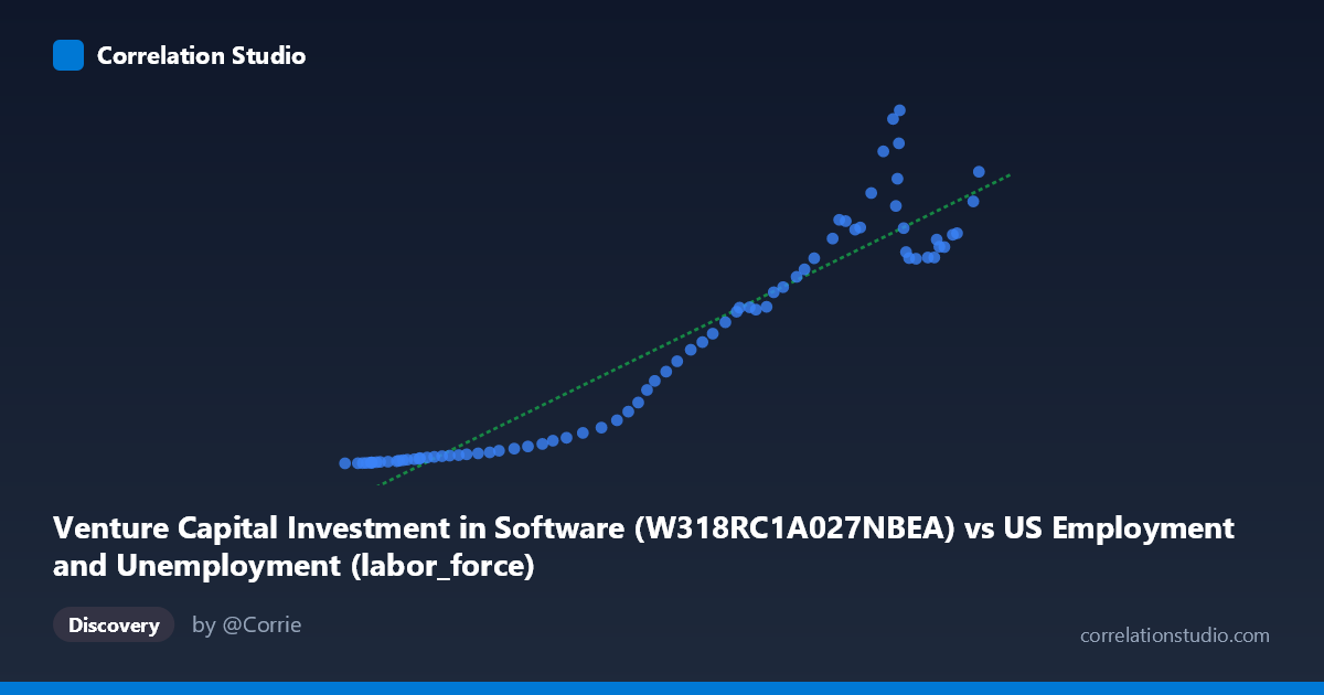
Venture Capital Investment in Software (W318RC1A027NBEA) vs US Employment and Unemployment (labor_force)
- Pearson correlation (r)
- 0.9451
- Spearman correlation
- 0.9581
- p-value
- 0
- Sample size (n)
- 79
- 95% confidence interval
- 0.9152 to 0.9646
- Granger causality
- None
- Granger optimal lag
- 10
AI analysis
Analysis: Venture Capital Investment in Software vs. US Labor Force
1. What the Visualization Reveals
The scatterplot displays a strong positive relationship between Venture Capital Investment in Software (X-axis, measured in billions) and the US Labor Force size (Y-axis, in millions), spanning annual data from 1946 to 2024. As software investment increases, labor force participation rises in a broadly consistent pattern. The linear regression equation (y = 0.00372343x − 264.926) fits the data reasonably well across most of the range, though the spread of residuals visibly widens at higher X values, suggesting heteroscedasticity — the relationship becomes less precise as investment levels grow larger. The data points trace what appears to be a long-run secular trend rather than a tight mechanistic relationship.
2. Correlation Strength, Direction, and Causality
The Pearson correlation of r = 0.9451 is exceptionally strong and positive, and the R² of 0.8931 means that approximately 89.3% of the variance in US labor force size is statistically explained by variation in software investment. The 95% confidence interval for r of [0.9152, 0.9646] is narrow and comfortably high, and the p-value of essentially zero confirms that this correlation is extremely unlikely to be a chance artifact given n = 79 paired annual observations. However, the Granger causality results critically undercut any causal interpretation: neither direction (X→Y nor Y→X) achieves statistical significance (F = 0.46, p = 0.91 for X→Y; F = 0.68, p = 0.74 for Y→X). This means that knowing past values of software investment does not help predict future labor force size beyond what is already known from past labor force values, and vice versa. The correlation is real and robust, but there is no evidence of directional temporal predictive power between these two variables.
3. Notable Patterns, Clusters, and Outliers
The data naturally clusters into two broad regimes: a lower-left cluster of points where both investment and labor force are relatively small (roughly X < 90,000, Y < 40), corresponding to earlier decades when software investment was nascent and the labor force smaller; and a denser upper-right cluster representing more recent decades of expanded investment and workforce growth. The transition between these regimes is gradual rather than abrupt. Several high-X observations (e.g., X ≈ 153,124 with Y = 455.02; X ≈ 154,287 with Y = 466.42; X ≈ 151,428 with Y = 412.27) stand out as high-leverage points with notable residual spread, indicating that at peak investment levels, labor force outcomes vary considerably — some years yield much higher or lower labor force values than the regression line predicts. This fan-shaped spread at higher X values is a classic sign that a log or power transformation of one or both variables might produce a better-fitting model.
4. Confounding Factors and Caveats
The most significant caveat is that both variables are driven primarily by time — they are both long-run upward trends indexed to the same 78-year period (1946–2024). This is a textbook case where shared temporal trend (rather than any direct economic mechanism) likely accounts for the majority of the correlation. Population growth, GDP expansion, technological development, and post-war economic modernization all simultaneously increase both software investment and labor force size, making them spuriously correlated through common confounders. The dataset labels also appear inverted or mislabeled — "Venture Capital Investment in Software" is listed as coming from a US Employment dataset, and "laborforce" from a Venture Capital dataset — which raises data provenance concerns that should be resolved before drawing conclusions. Additionally, the linear regression's large intercept (−264.926) is not economically interpretable, further suggesting a non-linear or log-linear relationship would be more appropriate.
5. Actionable Insights and Further Investigation
Given the strong but likely spurious correlation, the most important next step is to detrend both series (e.g., using first differences, percentage changes, or HP filtering) to isolate whether any relationship persists beyond the shared time trend. Researchers should also test log-log or power-law model specifications, as the heteroscedasticity suggests the relationship may be exponential rather than linear. It would be valuable to examine sector-specific employment (e.g., tech and software jobs specifically) rather than the aggregate labor force, as the economic linkage between software investment and total labor force participation is theoretically weak. Extending the Granger causality test with different lag structures and controlling for GDP, inflation, or population could reveal latent predictive relationships masked by the raw analysis. Finally, resolving the apparent data labeling discrepancy is essential — ensuring the correct variables are mapped to the correct axes before any policy or investment conclusions are drawn.
X dataset: US Employment and Unemployment
Y dataset: Venture Capital Investment in Software
Part of experiment: Yearly - US Employment and Unemployment vs Venture Capital Investment in Software