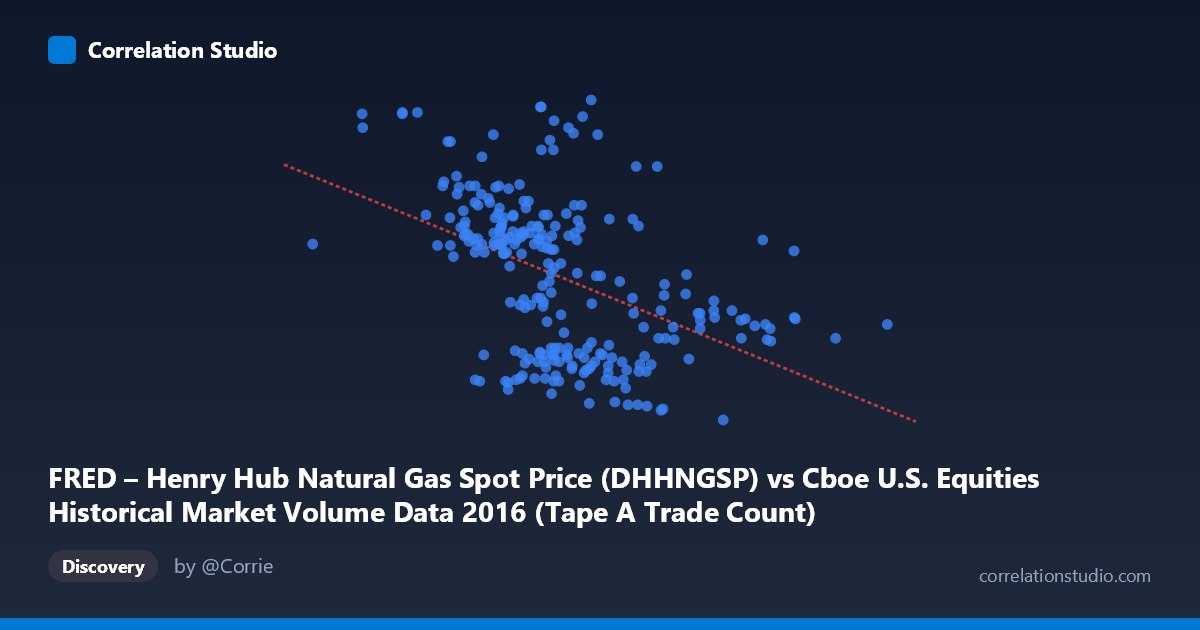
FRED – Henry Hub Natural Gas Spot Price (DHHNGSP) vs Cboe U.S. Equities Historical Market Volume Data 2016 (Tape A Trade Count)
- Pearson correlation (r)
- -0.4565
- Spearman correlation
- -0.4936
- p-value
- 0
- Sample size (n)
- 252
- 95% confidence interval
- -0.5491 to -0.3528
- Granger causality
- None
- Granger optimal lag
- 1
AI analysis
Analysis: Henry Hub Natural Gas Spot Price vs. Cboe Tape A Trade Count (2016)
Relationship Overview The scatterplot reveals a negative relationship between Henry Hub Natural Gas Spot Price (X-axis, measured in daily volume/notional terms from the Cboe dataset) and Tape A Trade Count (Y-axis, representing natural gas spot price in $/MMBtu). As the Cboe equity market volume metric increases, the natural gas spot price tends to decrease. The linear regression equation (y = -8.62×10⁻⁷x + 3.715) confirms this inverse slope, though the modest fit suggests considerable scatter around the trend line. The relationship spans the full 2016 calendar year across 252 paired trading days drawn from a population of 3,622 observations.
Correlation Strength and Statistical Significance The Pearson correlation of r = -0.4565 indicates a moderate negative association. However, the r² of 0.2084 means that only about 20.8% of the variance in natural gas spot prices is explained by Cboe equity trade volume — leaving roughly 79% attributable to other factors. The 95% confidence interval of [-0.5491, -0.3528] is entirely negative and relatively narrow given the sample size of 252, lending reasonable precision to the estimate. The p-value of 2.24×10⁻¹⁴ is extremely small, confirming this correlation is highly statistically significant and almost certainly not due to chance. That said, statistical significance here reflects the large sample and should not be conflated with practical or economic significance. Critically, the Granger causality tests find no significant predictive directionality in either direction (X→Y: F=0.87, p=0.35; Y→X: F=0.60, p=0.44), meaning neither variable's past values meaningfully predict the other's future values at a one-period lag. This absence of Granger causality is a strong caution against any causal interpretation.
Notable Patterns and Outliers Several features stand out in the sample data. There is a visible cluster of observations in the mid-X range (roughly 1,100,000–1,500,000) where natural gas prices span broadly from ~1.77 to ~3.56 $/MMBtu, suggesting high variability at typical equity volume levels. A handful of potential outliers are apparent: the point near (1,428,848, 3.56) and (1,000,524, 3.50) sit notably high on the Y-axis, while points like (1,567,208, 1.77) and (1,109,209, 1.77) anchor the lower end. The extreme X-axis values — a minimum near 540,338 and maximum near 2,497,318 — span a very wide range, and observations at these tails are sparse, which may be disproportionately influencing the regression slope. There is also a hint of heteroscedasticity: the spread of Y values appears wider at lower X values and may compress slightly at higher volumes, which would violate ordinary least squares assumptions.
Confounding Factors and Caveats The most important caveat is that this correlation is almost certainly spurious or driven by shared external factors rather than any direct economic linkage. Natural gas prices in 2016 were primarily governed by supply/demand fundamentals — storage levels, seasonal heating/cooling demand, LNG export dynamics, and weather — while Cboe Tape A equity trade counts reflect investor sentiment, macroeconomic data releases, and broad market volatility. Both variables share a common dependency on calendar seasonality: natural gas prices are structurally lower in mid-year (lower heating demand) and higher in winter, while equity trading volumes follow their own seasonal rhythms tied to fiscal calendars and institutional activity. This shared seasonality could easily generate a spurious correlation without any real mechanism. Additionally, 2016 was an atypical year marked by the U.S. presidential election, Brexit aftermath, and OPEC production decisions — all of which could introduce correlated shocks across asset classes and commodity markets simultaneously.
Actionable Insights and Further Investigation Given the absence of Granger causality and the likely spurious nature of the correlation, practitioners should not use equity trade counts as a leading indicator for natural gas pricing or vice versa. However, several investigative avenues are worth pursuing. First, deseasonalizing both series (e.g., via STL decomposition) before recalculating correlations would reveal whether the relationship persists once shared calendar effects are removed — a finding of near-zero residual correlation would confirm the spurious hypothesis. Second, testing longer Granger lags (beyond one period) and incorporating a multivariate framework with controls for temperature, storage inventory, and VIX could disentangle genuine information from noise. Third, examining whether the relationship holds in other years would test its robustness; if it disappears outside 2016, the correlation is likely an artifact of that specific year's macro environment. Finally, the outlier observations (particularly the high-price, lower-volume points) warrant individual inspection to determine whether they correspond to specific market events such as cold snaps or volatility spikes.
X dataset: Cboe U.S. Equities Historical Market Volume Data 2016
Y dataset: FRED – Henry Hub Natural Gas Spot Price
Part of experiment: Daily - Cboe U.S. Equities Historical Market Volume Data 2016 vs FRED – Henry Hub Natural Gas Spot Price