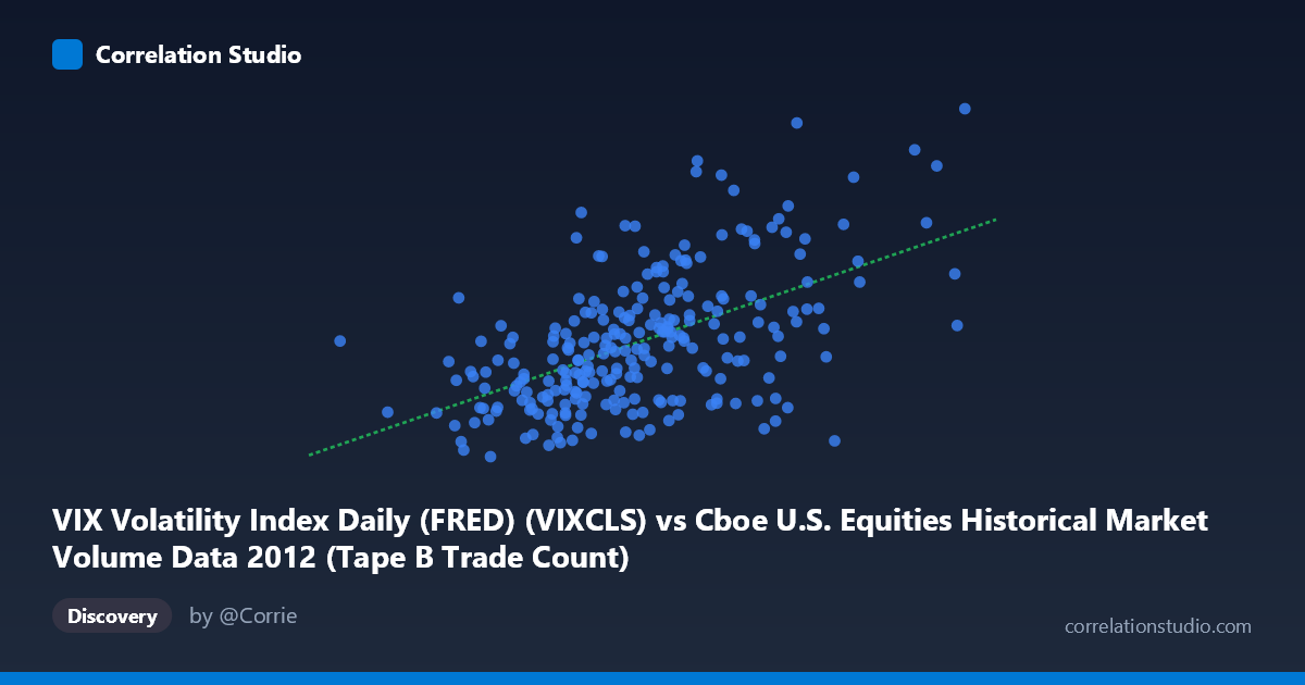
VIX Volatility Index Daily (FRED) (VIXCLS) vs Cboe U.S. Equities Historical Market Volume Data 2012 (Tape B Trade Count)
- Pearson correlation (r)
- 0.5454
- Spearman correlation
- 0.5296
- p-value
- 0
- Sample size (n)
- 250
- 95% confidence interval
- 0.4519 to 0.627
- Granger causality
- None
- Granger optimal lag
- 1
AI analysis
Analysis: VIX Volatility Index vs. Cboe Tape B Trade Count (2012)
Relationship Overview The scatterplot reveals a moderate positive relationship between the VIX Volatility Index and Cboe Tape B Trade Count across 250 trading days in 2012. As VIX values rise — indicating higher implied volatility and market fear — Tape B trade counts tend to increase correspondingly. This aligns intuitively with market microstructure theory: periods of elevated uncertainty typically drive higher trading activity as investors reposition, hedge, or react to news. The linear regression equation (y = 3.46829E-05x + 11.711) suggests that for every 10,000-unit increase in daily volume/notional measure on the X-axis, Tape B trade count rises by approximately 0.35 units, though the wide X-range (63,410 to 298,005) reflects substantial day-to-day variation in market activity.
Correlation Strength and Statistical Framing The Pearson correlation of r = 0.5454 indicates a moderate positive association, but the more sobering metric is r² = 0.2975 — meaning X explains only ~29.8% of the variance in Y, leaving roughly 70% attributable to other factors. The 95% confidence interval of [0.4519, 0.6270] is meaningfully above zero and relatively tight given N = 3,750, and the p-value of effectively 0 confirms this correlation is highly unlikely to be a statistical artifact. That said, statistical significance does not imply practical sufficiency: the relationship is real but far from deterministic. Critically, the Granger causality tests yield no significant directional predictive relationship in either direction (X→Y: F = 1.43, p = 0.23; Y→X: F = 0.11, p = 0.74), meaning that neither variable reliably predicts the other's future values at a 1-period lag. This cautions against any causal or forecasting interpretation of the correlation.
Notable Patterns, Clusters, and Outliers Several features stand out in the sample points. There is a dense central cluster between X ≈ 130,000–210,000 and Y ≈ 15–20, consistent with the mean values (X̄ = 175,526; Ȳ = 17.80), suggesting a core "normal trading regime" for 2012. However, notable vertical dispersion exists within this cluster — for instance, X values near 170,000–175,000 yield Y values ranging from 14.38 to 22.22 — indicating that similar volume levels can co-occur with very different VIX readings. There are potential outliers at the extremes: the point near (295,122, 18.43) represents an unusually high X value yet only a moderate Y, and several points around Y ≈ 23–26 (e.g., 211,236/23.56 and 197,126/24.27) suggest episodic volatility spikes. The upper-right and lower-right regions appear thinly populated, hinting at non-linearity or regime-dependent behavior.
Confounding Factors and Caveats Several important caveats apply. First, Tape B specifically covers NYSE American (AMEX) and regional exchange listings, meaning it represents a subset of total market activity rather than the full market, potentially introducing selection bias. Second, both VIX and trade counts are likely driven by common exogenous factors — macroeconomic announcements, earnings seasons, geopolitical events — creating spurious correlation without direct causation. Third, the 2012 time window is a single calendar year with specific macro characteristics (post-2011 European debt crisis, U.S. election cycle), limiting generalizability. Fourth, the Granger test used only a 1-period lag, which may be insufficient to capture delayed market responses. Finally, daily aggregation may mask intraday dynamics where the true relationship is more pronounced or more complex.
Actionable Insights and Further Investigation Practitioners and researchers should consider several follow-up directions. Regime-segmentation analysis — splitting the data into low, medium, and high VIX periods — could reveal whether the correlation strengthens during stress episodes, which would be more actionable for risk management. Testing multiple Granger lags (2–5 periods) would provide a more robust assessment of temporal predictability. Including additional explanatory variables such as S&P 500 returns, bid-ask spreads, or macroeconomic surprise indices could dramatically improve the explained variance beyond the current 29.8%. Extending the analysis across multiple years (especially including 2008–2009 or 2020) would test whether the VIX–volume relationship is stable or crisis-contingent. Finally, comparing Tape B results against Tape A (NYSE) and Tape C (Nasdaq) would clarify whether this relationship is exchange-specific or a broad market phenomenon.
X dataset: Cboe U.S. Equities Historical Market Volume Data 2012
Y dataset: VIX Volatility Index Daily (FRED)
Part of experiment: Daily - Cboe U.S. Equities Historical Market Volume Data 2012 vs VIX Volatility Index Daily (FRED)