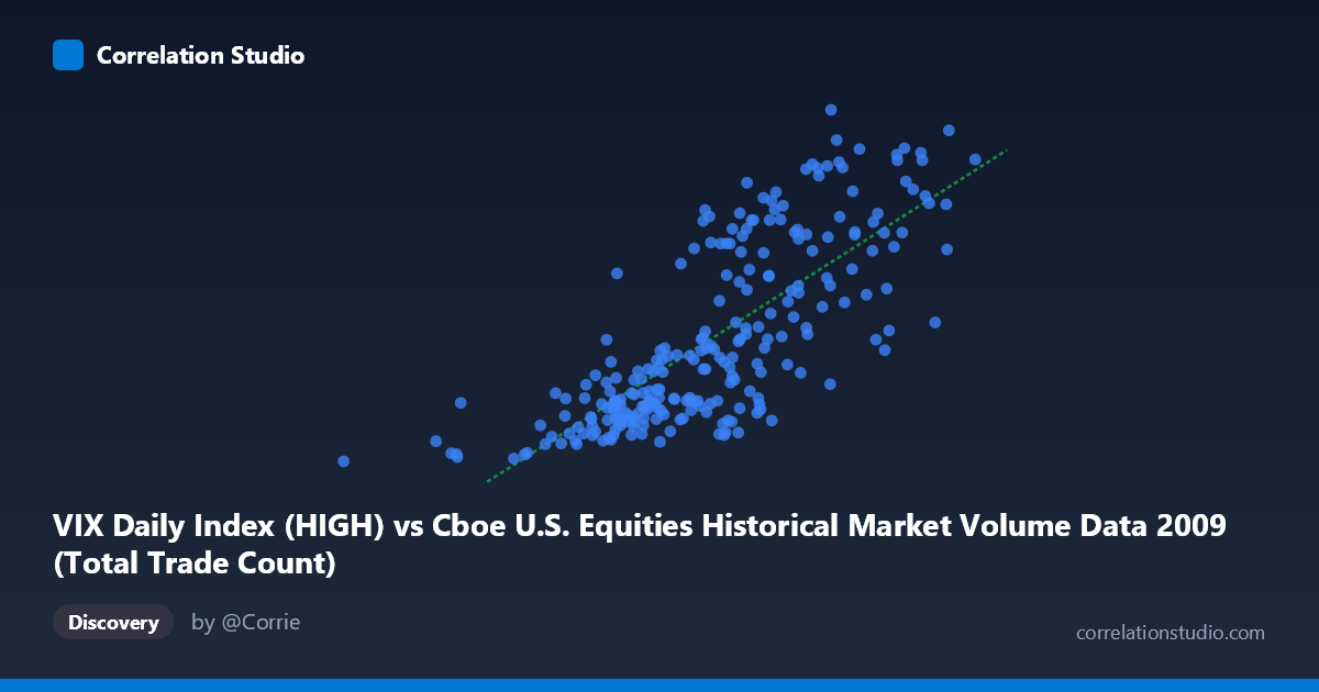
VIX Daily Index (HIGH) vs Cboe U.S. Equities Historical Market Volume Data 2009 (Total Trade Count)
- Pearson correlation (r)
- 0.7682
- Spearman correlation
- 0.7914
- p-value
- 0
- Sample size (n)
- 252
- 95% confidence interval
- 0.7122 to 0.8144
- Granger causality
- None
- Granger optimal lag
- 1
AI analysis
Analysis: VIX Daily Index (HIGH) vs. Total Trade Count (2009)
Relationship Overview The scatterplot reveals a moderately strong positive relationship between the CBOE VIX Daily High values and the Total Trade Count in U.S. equities markets throughout 2009. As VIX High values increase, total trade counts tend to rise correspondingly, which aligns intuitively with market microstructure theory: elevated volatility typically drives heightened trading activity as investors rebalance portfolios, execute hedges, or respond to rapidly changing price signals. The linear regression equation (y = 1.23392E-05x − 0.123352) confirms this positive slope, suggesting that each unit increase in VIX High is associated with a measurable increase in trade count volume.
Correlation Strength and Statistical Significance The Pearson correlation of r = 0.7682 indicates a strong positive association, and the R² of 0.5901 means that approximately 59% of the variance in Total Trade Count is explained by the VIX High level alone — a substantial but incomplete explanatory share, leaving ~41% attributable to other factors. The 95% confidence interval of [0.7122, 0.8144] is relatively narrow given the sample size (n = 252), lending confidence that this is a robust signal rather than a sampling artifact, and the p-value of effectively 0 confirms the relationship is statistically significant at any conventional threshold. However, the Granger causality results are notably absent of significance in either direction (X→Y: F = 0.2861, p = 0.593; Y→X: F = 0.1591, p = 0.690), meaning that despite the strong contemporaneous correlation, neither variable reliably predicts the other at a one-period lag. This is a critical distinction: VIX High and Trade Count move together, but one does not lead the other in a temporally predictive sense.
Notable Patterns, Clusters, and Outliers Several structural features are visible in the data. There is a dense cluster of points at lower X values (roughly VIX High between 2,000,000–3,000,000 and Trade Count between 20–35), corresponding to the more stable mid-to-late 2009 period as markets recovered from the financial crisis. A second, more dispersed upper cluster appears at higher VIX and trade count values, likely reflecting the elevated volatility environment of early 2009. A handful of outlier points — notably the extreme high-X observation at ~4,134,003 paired with a Trade Count of ~52 — sit at the far upper right and may represent specific market stress days. Conversely, the minimum X point (629,671, Trade Count ~19.67) anchors the lower left as a clear low-activity day. The spread around the regression line widens at higher X values, suggesting mild heteroscedasticity — variance in Trade Count increases with VIX High, which is a common feature in volatility-driven datasets.
Confounding Factors and Caveats Several important caveats limit causal interpretation. First, 2009 was an extraordinary year — spanning the tail of the global financial crisis and a historic market recovery — making patterns from this single year potentially unrepresentative of normal market conditions. Second, secular trends (e.g., the gradual normalization of volatility over 2009) may be driving both variables simultaneously, creating a spurious correlation through shared time-trend dependence rather than a true functional link. Third, market structure changes, algorithmic trading volumes, and exchange-specific routing behaviors could independently influence trade counts without any mechanistic connection to VIX. The axis labeling also warrants scrutiny: the X-axis references a "VIX Daily Index HIGH" column sourced from the market volume dataset, while the Y-axis references "Total Trade Count" sourced from the VIX dataset — suggesting these may be cross-joined fields that require careful verification of column provenance before drawing firm conclusions.
Actionable Insights and Further Investigation Practitioners and researchers should consider several follow-up steps. First, extending the time series beyond 2009 to multiple market regimes would test whether this r = 0.77 relationship holds in normal (low-volatility) environments or is specific to crisis periods. Second, decomposing the trade count by exchange, asset class, or trade size could reveal whether the VIX relationship is driven primarily by institutional hedging activity or retail panic trading. Third, applying non-linear models (e.g., log-log regression or quantile regression) may better capture the apparent heteroscedasticity and potential threshold effects at extreme VIX levels. Finally, given the lack of Granger causality, analysts should avoid building predictive trading signals based on lagged VIX readings to forecast next-day trade counts — the relationship is contemporaneous and likely driven by shared macro conditions, making same-day regime identification more appropriate than lag-based forecasting.
X dataset: Cboe U.S. Equities Historical Market Volume Data 2009
Y dataset: VIX Daily Index
Part of experiment: Daily - Cboe U.S. Equities Historical Market Volume Data 2009 vs VIX Daily Index