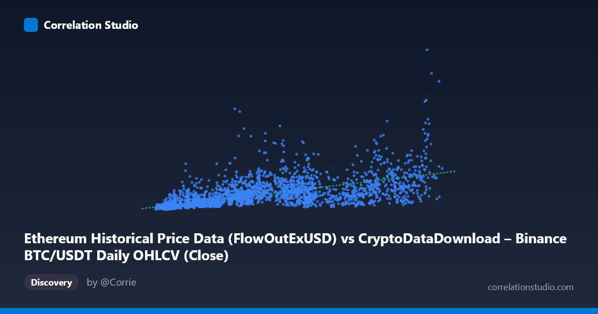
Ethereum Historical Price Data (FlowOutExUSD) vs CryptoDataDownload – Binance BTC/USDT Daily OHLCV (Close)

Pearson correlation (r): 0.6583
Spearman correlation: 0.8239
p-value: 0
Sample size (n): 3191
95% confidence interval: 0.6382 to 0.6776
Granger causality: Y → X
Granger optimal lag: 10
Time coverage: 2017-08-17 to 2026-05-20

AI analysis

Analysis: X–Y Relationship

1. Overview of the Relationship

The scatterplot shows a positive, moderately strong association between the X variable (labeled as an Ethereum "FlowOutExUSD" metric, though the sample data and range strongly resemble BTC/USDT closing prices) and the Y variable (labeled as BTC/USDT Close, though the magnitude—billions rather than tens of thousands—suggests it's actually a volume, market cap, or aggregated flow metric). As X increases, Y tends to increase as well, but the spread of Y-values widens considerably at higher X-values, indicating heteroscedasticity rather than a clean linear channel.

2. Strength, Direction, and Statistical Confidence

The Pearson correlation of r = 0.658 indicates a moderate-to-strong positive linear relationship, with r² = 0.433 meaning only 43.3% of the variance in Y is explained by X — the majority of Y's variability (56.7%) stems from other factors or nonlinear dynamics not captured by this simple linear fit. The tight 95% CI [0.638, 0.678] combined with a p-value ≈ 0 confirms this correlation is highly statistically significant and not a product of sampling noise, despite the large dataset (n=3,191) making even small correlations "significant" — here the effect size is genuinely moderate, not just statistically detectable.

The Granger causality results add an important asymmetry: Y Granger-causes X (F=2.039, p=0.026) at a 10-period lag, while X does NOT Granger-cause Y (p=0.161). This suggests that past values of Y contain predictive information about future X, but not vice versa — practically, this implies Y-side dynamics (e.g., volume/flow shocks) may lead price/X movements with a ~10-day lag, rather than X driving Y. This is a purely statistical/temporal precedence result, not proof of causal mechanism.

3. Notable Patterns and Non-linear Features

The sample points reveal a clear fan-shaped/heteroscedastic pattern: at low X (under ~15,000), Y values are tightly clustered in the tens-of-millions range, but as X climbs past 50,000–80,000, Y disperses wildly — ranging from ~300M to over 1.6B for similar X-values (e.g., X≈62,432 → Y≈1.69B, while X≈83,890 → Y≈628M). This divergence, combined with the note that Spearman's ρ exceeds Pearson's r, strongly suggests a non-linear (likely logarithmic or power-law) relationship better fits the data than the linear model. Several high-leverage outliers exist — points like (36,445 → 1.31B) and (53,788 → 1.40B) sit well above the regression line, while (110,188 → 605M) sits below it, indicating the linear fit systematically misprices both tails of the X distribution.

4. Confounding Factors and Caveats

Given the mismatched axis labels/scales (X described as an ETH flow metric but ranging like BTC price; Y described as BTC close but scaled like a large-cap volume metric), there is likely a data-labeling or column-mapping error that should be resolved before drawing domain conclusions. Additionally, both series span 2017–2026, a period encompassing multiple bull/bear cycles, halving events, and macro shocks (COVID, rate hikes) — this creates regime-dependent correlation where the relationship may be driven by shared trends (both assets rising in bull markets) rather than a direct mechanical link. Time-series data is also prone to autocorrelation, inflating apparent significance in both the Pearson test and the Granger test if not properly differenced.

5. Recommendations for Further Investigation

1. Verify column/axis labels — confirm which series is actually price vs. volume/flow before interpreting economic meaning. 2. Fit non-linear models (log-log, power law) given the Spearman/Pearson divergence and fan-shaped residuals; compare R² against the linear baseline. 3. Segment by market regime (bull/bear/sideways) to check if correlation strength is stable or regime-dependent. 4. Test stationarity and differencing before trusting Granger causality results — run the test on returns/log-differences rather than levels to rule out spurious causality from shared trends. 5. Investigate the 10-period lag mechanism — if Y→X causality holds after robustness checks, explore whether this reflects a genuine leading indicator relationship (e.g., volume/flow surges preceding price moves) worth building into a predictive trading signal.

X dataset: CryptoDataDownload – Binance BTC/USDT Daily OHLCV

Y dataset: Ethereum Historical Price Data

Part of experiment: Bitcoin - CryptoDataDownload – Binance BTC/USDT Daily OHLCV vs Ethereum Historical Price Data