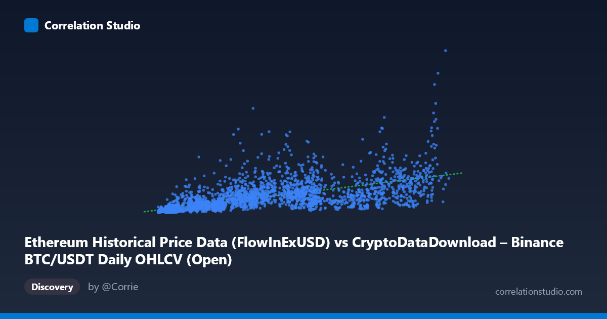
Ethereum Historical Price Data (FlowInExUSD) vs CryptoDataDownload – Binance BTC/USDT Daily OHLCV (Open)
- Pearson correlation (r)
- 0.6577
- Spearman correlation
- 0.8179
- p-value
- 0
- Sample size (n)
- 3191
- 95% confidence interval
- 0.6375 to 0.6769
- Granger causality
- Y → X
- Granger optimal lag
- 10
- Time coverage
- 2017-08-17 to 2026-05-20
AI analysis
Analysis: BTC/USDT Flow vs. Price Relationship
1. What the Visualization Reveals
The scatterplot shows a moderate positive relationship between two variables that—based on the metadata—appear to be mislabeled or conflated during dataset merging (the X-axis column references "FlowInExUSD" while described as Ethereum data, but the title references BTC/USDT OHLCV; the Y-axis is labeled as an "Open" price from the same Binance BTC dataset). Setting aside the labeling ambiguity, the data reveals a general upward trend: as X increases, Y tends to increase as well, but with substantial scatter rather than a tight linear band. This spread is visible in the sample points—for instance, X≈57,000 corresponds to Y values ranging from 685M to 1.79B, indicating that X alone does not tightly determine Y.
2. Strength, Direction, and Predictive Direction
The Pearson correlation (r = 0.658) indicates a moderate-to-strong positive relationship, but r² = 0.4325 means only 43% of the variance in Y is explained by X—the majority (57%) is driven by other factors, volatility, or nonlinearity not captured by this simple linear relationship. The 95% CI [0.6375, 0.6769] is tight given the large sample size (n=3,191), and the p-value of ~0 confirms the correlation is highly statistically significant and not due to chance. However, statistical significance here reflects sample size more than practical predictive strength.
The Granger causality results are notable: Y Granger-causes X, not the reverse (Y→X: F=2.60, p=0.0038 vs. X→Y: F=1.51, p=0.128, non-significant). This suggests that past values of Y have predictive power for future values of X at a 10-period lag, but not vice versa. This is an important asymmetry—correlation alone would not reveal this directional, time-lagged dependency, and it implies Y may be a leading indicator for X in this dataset.
3. Notable Patterns and Outliers
The data shows heteroscedasticity: variance in Y increases substantially as X increases, creating a "fan" or "cone" shape typical of financial/price data where percentage volatility compounds with price level. Several sample points show extreme Y-values relative to nearby X (e.g., X≈57,037 → Y≈1.79B, while X≈57,635 → Y≈685M)—two X values very close together yield wildly different Y outcomes, reinforcing that X is a weak-to-moderate predictor at any single point. The note that Spearman ρ exceeds Pearson r strongly suggests the true relationship is monotonic but non-linear—likely logarithmic, power-law, or exponential, consistent with price/volume data that often follows log-normal distributions.
4. Confounding Factors and Caveats
Several caveats apply: (a) Metadata inconsistency — the axis labels/descriptions suggest possible data merging errors between BTC and ETH datasets, which should be verified before drawing asset-specific conclusions; (b) Time-series autocorrelation — both series span 2017–2026 and are almost certainly non-stationary (trending), which can inflate Pearson correlation and distort Granger causality tests; differencing or returns-based analysis is needed to validate causality claims; (c) Common macro drivers — crypto asset prices are heavily influenced by shared external factors (Bitcoin dominance, regulatory news, macro liquidity, exchange flows) that could create spurious correlation between two related but distinct instruments; (d) Heteroscedasticity violates linear regression assumptions, meaning the reported R² and regression coefficients may be unreliable for large X values.
5. Actionable Insights
1. Verify data provenance — confirm whether X and Y are correctly attributed to BTC and/or ETH before further modeling, given the apparent labeling conflict. 2. Test log-log or log-linear transformations — given Spearman Pearson and the heteroscedastic fan pattern, refitting with log(X) and log(Y) will likely substantially improve R² and normalize variance. 3. Use returns/differenced series for Granger causality to rule out spurious causality from shared trends; re-run tests on stationary transformations. 4. Investigate the 10-period lag — examine what economic/market mechanism (e.g., order flow, arbitrage lag) could explain Y leading X, and backtest this as a potential trading signal.
X dataset: CryptoDataDownload – Binance BTC/USDT Daily OHLCV
Y dataset: Ethereum Historical Price Data
Part of experiment: Bitcoin - CryptoDataDownload – Binance BTC/USDT Daily OHLCV vs Ethereum Historical Price Data