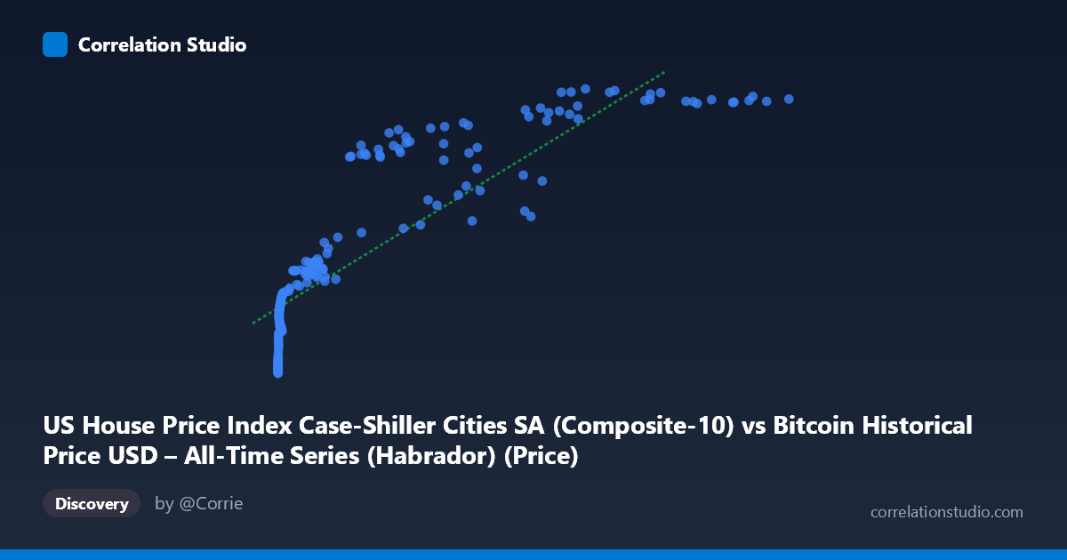
US House Price Index Case-Shiller Cities SA (Composite-10) vs Bitcoin Historical Price USD – All-Time Series (Habrador) (Price)
- Pearson correlation (r)
- 0.8638
- Spearman correlation
- 0.9703
- p-value
- 0
- Sample size (n)
- 191
- 95% confidence interval
- 0.8227 to 0.8959
- Granger causality
- None
- Granger optimal lag
- 2
- Time coverage
- 2010-08-01 to 2026-06-01
- Recomputed on refreshed data
- 2026-10-24 (r was 0.8592)
AI analysis
Analysis: Bitcoin Price vs. US House Price Index (Case-Shiller Composite-10)
1. Relationship Overview
The scatterplot depicts a strong positive association between Bitcoin's historical USD price (X-axis) and the Case-Shiller Composite-10 Home Price Index (Y-axis). The relationship is distinctly non-linear: at low Bitcoin prices (under ~$1,000), the Case-Shiller index clusters tightly in the 150–210 range, while as Bitcoin climbs into the tens of thousands, the index rises and compresses toward an upper ceiling near 350–365. This produces a curve resembling a logarithmic or saturating growth pattern rather than a straight line — consistent with the fact that Bitcoin's X-values span nearly six orders of magnitude (0.06 to 118,670) while Y only ranges from 149 to 364.
2. Strength, Direction, and Statistical Confidence
The Pearson correlation (r = 0.855, r² = 0.731) indicates a strong positive linear relationship, with the linear model explaining about 73% of the variance in Y. The 95% CI [0.811, 0.890] is narrow and does not cross zero, and the p-value is effectively 0, so we can be highly confident a real statistical association exists in this sample — this is not noise. However, the note that Spearman's ρ exceeds Pearson's r is a strong hint that a monotonic but curved (log/power) relationship fits better than a straight line, meaning the "true" explanatory power is likely understated by the linear r². Critically, Granger causality tests show no predictive direction in either direction (p ≈ 0.79 both ways at 9 lags) — despite the strong contemporaneous correlation, neither series' past values help forecast the other's future values. This is a classic case of correlation without demonstrated temporal causality.
3. Notable Patterns and Features
- Log-scale clustering: The vast majority of X-values are below 100,000, with a dense cluster under 10,000 and a sparser tail extending to 118,670 — typical of Bitcoin's exponential growth history. - Ceiling effect in Y: The Case-Shiller index appears to plateau near 350–365 even as Bitcoin prices continue rising past $60,000–$118,000, suggesting the relationship flattens (saturates) at high X values — hence the log-fit suggestion. - Tight low-end cluster: Nearly identical low Y-values (149–160) for a wide range of very small X-values (0.06 to ~20) suggest an early period (likely 2010–2013) where Bitcoin was negligible in price and home prices were still near post-financial-crisis lows. - No obvious discrete outliers — the pattern is a smooth, continuous curve rather than scattered noise, consistent with two macro trending series.
4. Confounding Factors and Caveats
This is very likely a spurious/confounded correlation driven by shared time trends, not a causal economic link. Both series have risen dramatically over roughly the same 2010–2026 window due to entirely different mechanisms: Bitcoin's adoption/speculative cycles vs. housing market dynamics (low interest rates, post-2008 recovery, pandemic-era demand). Any two long-term upward-trending time series will show high correlation purely by virtue of time itself acting as a lurking variable. The lack of Granger causality reinforces this: if Bitcoin genuinely influenced housing prices (or vice versa) mechanistically, we'd expect lagged predictive power, which is absent. Additionally, the data aren't true "paired" observations of interacting variables — they're two independent macro series merely sampled over overlapping calendar dates.
5. Suggested Next Steps
- De-trend both series (e.g., using year-over-year growth rates or differencing) and re-run the correlation; genuine co-movement should survive de-trending, whereas spurious trend-driven correlation should largely disappear. - Fit and compare a log-linear or power-law model (e.g., Y vs. log(X)) given the Spearman/Pearson discrepancy — this should meaningfully improve fit over the naive linear R². - Test for cointegration (e.g., Engle-Granger) rather than relying on simple correlation, since both are non-stationary trending series. - Consider third-variable analysis: control for macro drivers like Fed interest rates, M2 money supply, or inflation, which plausibly drive both housing prices and speculative asset prices (including Bitcoin) simultaneously. - Treat this correlation as descriptive/historical rather than predictive or actionable for trading/investment decisions, given the Granger causality results explicitly rule out forecasting value in either direction.
X dataset: Bitcoin Historical Price USD – All-Time Series (Habrador)
Y dataset: US House Price Index Case-Shiller Cities SA
Part of experiment: Bitcoin - Bitcoin Historical Price USD – All-Time Series (Habrador) vs US House Price Index Case-Shiller Cities SA