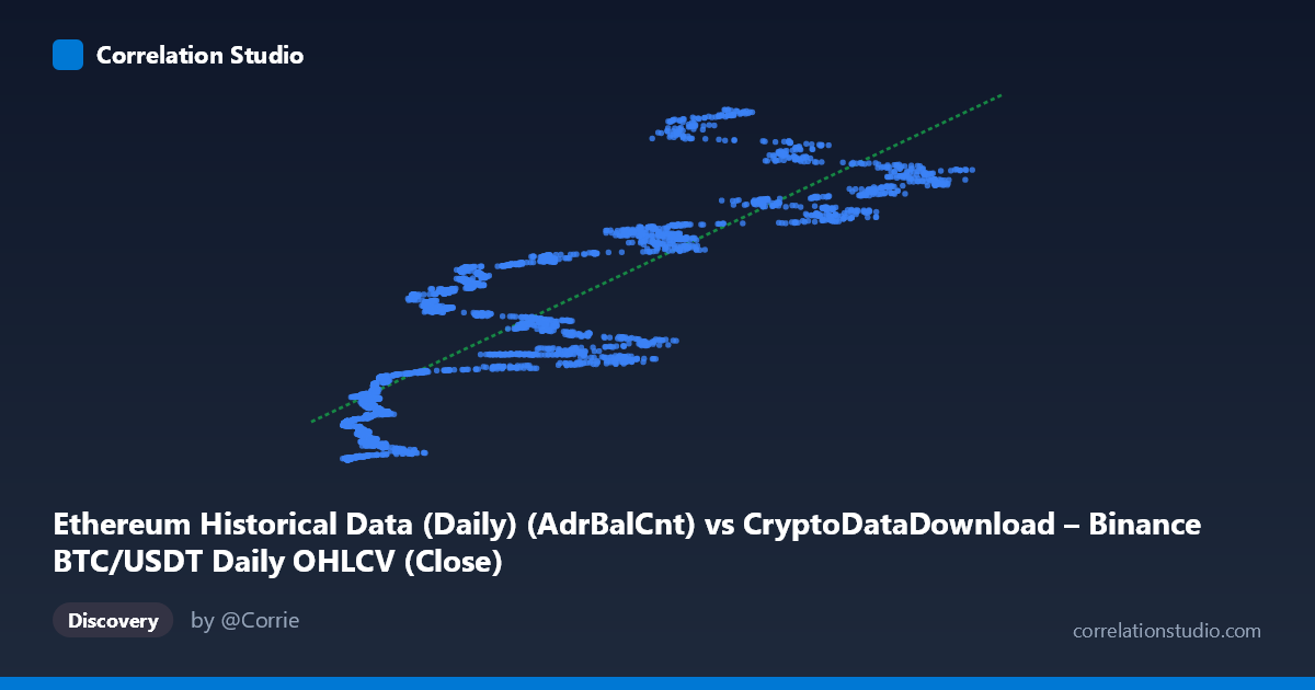
Ethereum Historical Data (Daily) (AdrBalCnt) vs CryptoDataDownload – Binance BTC/USDT Daily OHLCV (Close)

Pearson correlation (r): 0.8574
Spearman correlation: 0.8875
p-value: 0
Sample size (n): 3191
95% confidence interval: 0.8479 to 0.8663
Granger causality: None
Granger optimal lag: 10

AI analysis

Analysis of the Scatterplot Relationship

1. Overview of the Visualization

The scatterplot displays a clear positive, upward-sloping relationship between the X variable (labeled as Ethereum address balance count, though the surrounding metadata suggests this may actually be a mislabeled BTC/ETH-related metric) and Y (labeled as BTC/USDT closing price). As X increases from roughly 3,000 to 125,000, Y rises from near 3 million to nearly 193 million. The scatter shows a fairly consistent linear trend, with points fanning out somewhat more widely at higher X values, indicating increasing variance (heteroscedasticity) as the independent variable grows.

2. Strength, Direction, and Statistical Confidence

The correlation coefficient (r = 0.857) indicates a strong positive linear relationship. The r² value of 0.735 means approximately 73.5% of the variance in Y is statistically explained by X — a substantial but not complete relationship, leaving about 26.5% of Y's variance driven by other factors, noise, or nonlinear dynamics not captured by this simple linear model. The 95% confidence interval [0.848, 0.866] is narrow, reflecting the large sample size (n=3,191) and giving strong confidence that the true population correlation lies within this tight band. The p-value of ~0 confirms this correlation is highly statistically significant and not due to random chance.

Critically, the Granger causality test reveals no significant predictive direction in either direction (X→Y: p=0.407; Y→X: p=0.200). This is an important caveat: despite the strong contemporaneous correlation, neither variable reliably predicts future values of the other at the tested lag structure (10 periods). This suggests the relationship may be driven by a shared underlying factor (e.g., overall crypto market cycles, macroeconomic sentiment, or a common time trend) rather than one variable causally leading the other in a temporal sense.

3. Patterns, Clusters, and Outliers

Several notable features emerge from the sample data: - Low-X cluster (X < 10,000): These points show high variability in Y (ranging from ~3 million to ~48 million) despite similar X values, suggesting a noisy or possibly nonlinear relationship in this regime — small changes in X correspond to large swings in Y. - Mid-range clustering (X: 20,000–70,000): Points here follow the linear trend more tightly, suggesting the model fits best in this range. - High-X tail (X 80,000): Y values climb steeply and inconsistently (e.g., X≈78,231 → Y≈189.9M, but X≈81,447 → Y≈190.6M while X≈90,628 → Y≈170.8M), hinting at potential ceiling effects or regime changes at the top of the range. - The overall shape suggests a possible log-linear or power-law relationship rather than strictly linear, given the compressed low-X variance and expanded high-X variance — worth testing.

4. Confounding Factors and Caveats

Several caveats apply: - Metadata inconsistency: The dataset descriptions are contradictory/mismatched (X labeled as Ethereum address count but described as BTC/USDT OHLCV; Y labeled as BTC close price but described as Ethereum network metrics). This makes it unclear which variables are truly being compared, and any causal interpretation should be treated cautiously until this is resolved. - Common trend confounding: Both crypto prices and on-chain metrics (like address counts) tend to trend upward over multi-year periods due to overall market growth/adoption. This shared time trend can inflate correlation without genuine causal linkage — consistent with the null Granger causality result. - Non-stationarity: Financial and blockchain time series are typically non-stationary (trending, volatile), which can produce spurious correlations. The Granger test's null result may partly reflect this, or the true relationship may operate at different lag structures than the 10-period lag tested. - Heteroscedasticity: Growing variance at high X values violates linear regression assumptions, meaning R² and prediction intervals may be less reliable at the extremes.

5. Actionable Recommendations

1. Verify variable identities/metadata — resolve the labeling discrepancy before drawing substantive conclusions about what's actually being measured. 2. Test alternative functional forms (log-log, power law) given the heteroscedastic fan pattern — a log transformation may yield a better-fitting, more homoscedastic model. 3. Difference or detrend the series before re-running Granger causality, since both series likely share a non-stationary trend that could mask or distort true lead-lag relationships. 4. Test additional lag structures in Granger causality (e.g., 1-5 periods, or 20-30) since crypto markets can have both very short-term and longer-term dependencies not captured at lag 10. 5. Segment analysis by time period (e.g., bull vs. bear market phases) to check whether the relationship strength or direction changes across different market regimes, which is common in crypto data.

X dataset: CryptoDataDownload – Binance BTC/USDT Daily OHLCV

Y dataset: Ethereum Historical Data (Daily)

Part of experiment: Bitcoin - CryptoDataDownload – Binance BTC/USDT Daily OHLCV vs Ethereum Historical Data (Daily)