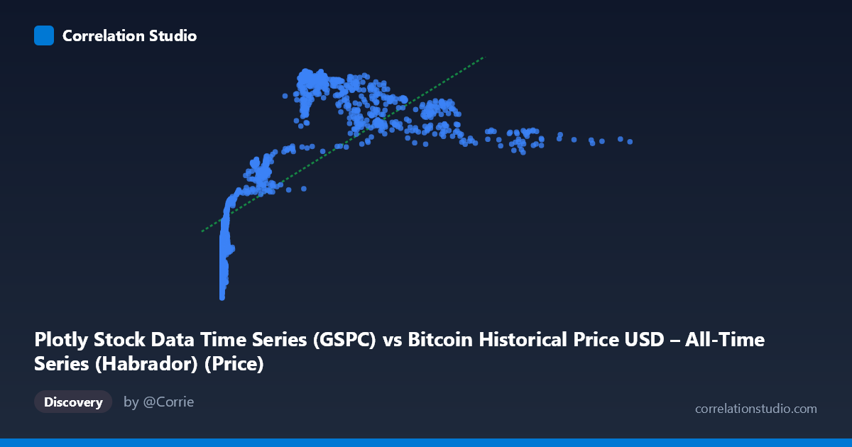
Plotly Stock Data Time Series (GSPC) vs Bitcoin Historical Price USD – All-Time Series (Habrador) (Price)
- Pearson correlation (r)
- 0.7281
- Spearman correlation
- 0.8491
- p-value
- 0
- Sample size (n)
- 1415
- 95% confidence interval
- 0.7026 to 0.7517
- Granger causality
- None
- Granger optimal lag
- 1
AI analysis
Analysis: Bitcoin (X) vs. GSPC/S&P 500 (Y) Price Series
1. What the Visualization Reveals
The scatterplot shows a positive but clearly non-linear relationship between the two price series. At low X values (near 0), Y ranges widely from ~1,050 to ~1,470 — indicating that when Bitcoin prices were near zero (the early historical period), the S&P 500 was already climbing through a range of values. As X increases past ~100–700, Y rises more steeply and then appears to plateau or saturate around 1,950–2,100, with less spread. This pattern — steep initial variance at low X, followed by compression at higher X — is characteristic of a logarithmic or square-root relationship rather than a straight line, which matches the note that Spearman's ρ exceeds Pearson's r.
2. Strength, Direction, and Statistical Confidence
The Pearson correlation (r = 0.728) indicates a moderately strong positive linear association, with r² = 0.530 meaning the linear model explains only 53% of the variance in Y — leaving nearly half unexplained by a straight-line fit. The tight 95% CI [0.703, 0.752] and p-value of 0 confirm this correlation is highly statistically robust and not due to chance, given the large sample (n=1,415). However, statistical significance here reflects the strength of association, not causation — and this is reinforced by the Granger causality tests: neither direction (X→Y: p=0.138; Y→X: p=0.628) shows significant predictive power at 1-lag. This means Bitcoin price changes do not reliably precede S&P 500 movements, or vice versa, in a temporal/predictive sense — the correlation is likely driven by both series trending upward over the same historical window (2010–2016) rather than any direct mechanistic link.
3. Notable Patterns and Structure
Several distinct features stand out: - Dense cluster near X≈0: Many points sit at X < 15 with Y spanning 1,050–1,470, reflecting Bitcoin's early years when its price was negligible while the S&P 500 moved independently through its own bull market. - A secondary "elbow" cluster around X≈200–320, Y≈1,940–2,100: suggesting a period where Bitcoin prices rose into the hundreds while the S&P 500 had already reached a higher plateau. - A flattening/high-X tail (X≈400–700): Y values compress into a narrower 1,780–2,000 band, indicating diminishing returns — large Bitcoin price increases correspond to comparatively small S&P 500 gains, consistent with a logarithmic curve. - No obvious extreme outliers, but the low-X vertical spread (1,050–1,470 at X≈0–15) is the most visually striking deviation from linearity.
4. Confounding Factors and Caveats
This is almost certainly a spurious or coincidental correlation driven by a shared confound: time. Both series are time-indexed and both trended upward from 2010–2016 (Bitcoin due to adoption/speculation growth from near-zero; the S&P 500 due to the post-2008 recovery bull market). Correlating two non-stationary trending time series will produce inflated correlation coefficients even absent any real relationship — a classic case of "spurious regression." The lack of Granger causality strongly supports this interpretation. Additionally, the vastly different scales and volatility regimes (Bitcoin's exponential growth vs. S&P's steady climb) mean a linear Pearson correlation is a poor descriptive tool here regardless of causal interpretation.
5. Recommendations for Further Investigation
- Detrend or difference both series (e.g., use daily/monthly returns instead of price levels) and recompute correlation — this is essential to rule out spurious trend-driven correlation. - Fit non-linear models (log-log or polynomial regression) given the Spearman/Pearson divergence; a log transformation of X may substantially improve fit. - Re-run Granger causality on stationary (differenced) series, since Granger tests on non-stationary price levels are unreliable and prone to false negatives/positives. - Treat the current r/r² as descriptive of co-movement over this historical window only, not as evidence of any economic or predictive relationship between Bitcoin and equity markets.
X dataset: Bitcoin Historical Price USD – All-Time Series (Habrador)
Y dataset: Plotly Stock Data Time Series
Part of experiment: Bitcoin - Bitcoin Historical Price USD – All-Time Series (Habrador) vs Plotly Stock Data Time Series