S&P 500 Daily Time Series since 1927 (GitHub fja05680) (Date) (Volume) vs Cboe U.S. Equities Historical Market Volume Data 2014 (Tape C Notional)
- Pearson correlation (r)
- 0.8626
- Spearman correlation
- 0.8099
- p-value
- 0
- Sample size (n)
- 252
- 95% confidence interval
- 0.8272 to 0.8912
- Granger causality
- None
- Granger optimal lag
- 10
AI analysis
Scatterplot Analysis: S&P 500 Volume vs. Cboe Tape C Notional Value (2014)
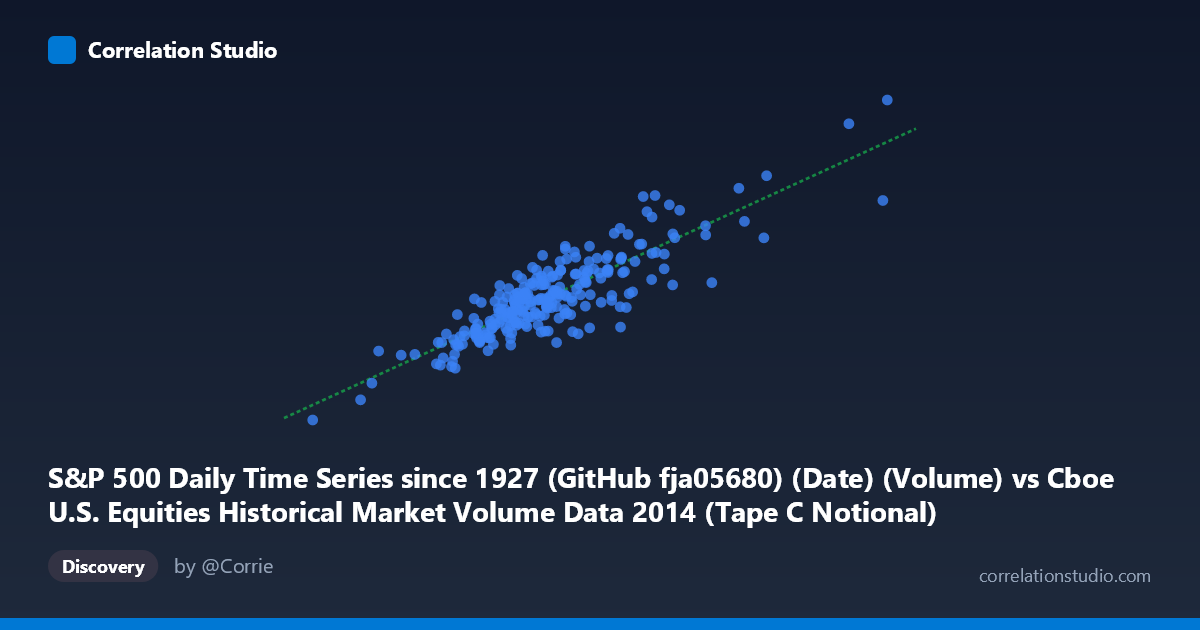
Relationship Overview The scatterplot reveals a strong positive linear relationship between S&P 500 daily trading volume and Cboe Tape C notional value across 2014. As daily volume increases, the notional value of Tape C trades rises correspondingly, which is intuitively sensible — higher share volumes traded generally translate into greater dollar-denominated notional activity. The data points form a reasonably tight upward-sloping band, with the regression line y = 0.5896x + 4.99×10⁸ capturing the central tendency well. The slope indicates that each additional unit of volume is associated with approximately $0.59 in additional notional value, with a substantial baseline intercept reflecting fixed notional activity independent of volume fluctuations.
Correlation Strength and Statistical Significance The Pearson correlation of r = 0.8626 indicates a strong positive association, and the coefficient of determination r² = 0.7441 means that roughly 74.4% of the variance in Tape C notional value is explained by S&P 500 volume alone — a meaningfully high proportion for financial market data. The 95% confidence interval of [0.8272, 0.8912] is relatively narrow given the sample size of n = 252, and the p-value of essentially zero confirms this relationship is not attributable to chance in a population of N = 3,686 observations. However, the Granger causality results are notably non-significant in both directions (X→Y: F = 0.758, p = 0.669; Y→X: F = 0.801, p = 0.628) with an optimal lag of 10 periods. This means that while the two variables are strongly contemporaneously correlated, neither reliably predicts the other in a temporal, lead-lag sense — the relationship appears to be concurrent and symmetric rather than directionally causal.
Patterns, Clusters, and Outliers The sample points reveal several notable structural features. The bulk of observations cluster in the mid-range (X: ~4.0–5.5 billion, Y: ~2.8–4.0 billion), consistent with typical 2014 trading days. However, there are visible high-volume outliers in the upper-right region — points such as (7.18B, 5.07B) and (6.77B, 4.34B) — likely corresponding to elevated volatility events, index rebalancing days, or options expiration periods. Conversely, the lower-left point at approximately (1.96B, 1.42B) is a pronounced low-volume outlier, potentially a holiday-shortened session or an anomalous low-activity day. There is also some vertical spread at mid-range X values (e.g., two points near X ≈ 5.7B diverge significantly in Y: ~3.2B vs. ~4.0B), suggesting that volume alone does not fully determine notional value — price levels and average trade size also matter.
Confounding Factors and Caveats Several important caveats temper interpretation. First, notional value is a product of both volume and price, so rising equity prices throughout 2014 would inflate notional values even on moderate-volume days, potentially inflating the correlation. Second, the axis labeling appears inverted in the dataset metadata — Volume is listed as the X variable from the S&P 500 dataset while Tape C Notional is the Y from the Cboe dataset, but the column sourcing descriptions are cross-referenced, warranting verification of which variable is truly on each axis. Third, the lack of Granger causality despite high contemporaneous correlation suggests both variables may be jointly driven by a third factor — such as broad market volatility (VIX), macroeconomic news events, or intraday liquidity conditions — making the correlation largely a reflection of shared external drivers rather than a direct structural link. Seasonality and end-of-quarter effects in 2014 may also cluster observations in ways that artificially strengthen the linear fit.
Actionable Insights and Further Investigation Practitioners should not use historical volume as a leading indicator for notional value (or vice versa) given the absence of Granger causality — any trading or risk model relying on a predictive lag between these series would lack empirical support. Instead, VIX or realized volatility should be explored as a potential common driver explaining the residual 25.6% of variance. It would be valuable to disaggregate the data by market regime (e.g., high-VIX vs. low-VIX periods) to test whether the correlation strengthens or weakens under stress conditions. Investigating the identified outlier days specifically could reveal whether they correspond to systematic events (FOMC announcements, options expiry, index reconstitution) that warrant separate modeling. Finally, extending the analysis beyond 2014 would test whether this r² of 0.74 is stable across different market cycles or is a feature specific to the relatively low-volatility 2014 environment.
X dataset: Cboe U.S. Equities Historical Market Volume Data 2014
Y dataset: S&P 500 Daily Time Series since 1927 (GitHub fja05680) (Date)
Part of experiment: Daily - Cboe U.S. Equities Historical Market Volume Data 2014 vs S&P 500 Daily Time Series since 1927 (GitHub fja05680) (Date)