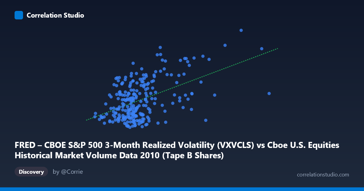
FRED – CBOE S&P 500 3-Month Realized Volatility (VXVCLS) vs Cboe U.S. Equities Historical Market Volume Data 2010 (Tape B Shares)
- Pearson correlation (r)
- 0.4985
- Spearman correlation
- 0.3691
- p-value
- 0
- Sample size (n)
- 252
- 95% confidence interval
- 0.3995 to 0.586
- Granger causality
- Y → X
- Granger optimal lag
- 1
AI analysis
Analysis: CBOE S&P 500 3-Month Realized Volatility vs. Tape B Shares Volume (2010)
Relationship Overview
The scatterplot reveals a moderate positive relationship between CBOE S&P 500 3-month realized volatility (VXVCLS, on the X-axis) and Tape B share volume (Y-axis) across 252 trading days in 2010. As realized volatility increases, Tape B share volume tends to rise as well, consistent with the well-established financial market principle that heightened uncertainty drives greater trading activity. The linear regression equation (y = 5.13×10⁻⁸x + 19.06) suggests a baseline volume level even at low volatility, with a gradual upward slope as volatility climbs. The relationship is clearly positive but visibly noisy, indicating that volatility alone is far from a complete explanation for daily volume behavior.
Correlation Strength and Statistical Significance
The Pearson correlation of r = 0.4985 reflects a moderate positive association, but the more informative metric is r² = 0.2485 — meaning realized volatility explains only ~24.9% of the variance in Tape B share volume. Roughly three-quarters of volume variation is driven by other forces entirely. The 95% confidence interval for r of [0.3995, 0.5860] is reasonably tight given n = 252, and the p-value of effectively zero confirms this correlation is highly statistically significant and not a sampling artifact. However, statistical significance should not be conflated with practical magnitude — a quarter of explained variance, while meaningful, leaves substantial unexplained dynamics.
The Granger causality results are particularly telling: Y Granger-causes X (F = 7.62, p = 0.006) with a 1-period optimal lag, while X does not significantly Granger-cause Y (F = 3.04, p = 0.082). This is a counterintuitive but important finding — Tape B share volume appears to have stronger temporal predictive power over subsequent realized volatility than vice versa. In practical terms, elevated Tape B trading activity today may signal rising volatility tomorrow, rather than volatility mechanically driving volume in a forward-looking sense. This inverts a naive causal assumption and suggests volume may be a leading indicator worth monitoring.
Notable Patterns, Clusters, and Outliers
The scatterplot shows a visible central cluster in the X range of roughly 70–150 million (moderate volatility) with Y values concentrated between 19–27, forming a dense core. Above X ≈ 180 million, the data becomes increasingly sparse but the upward trend becomes more pronounced, with several high-leverage points in the upper right (e.g., the observations near X = 316M, Y = 36.6 and X = 255M, Y = 37.4) that appear to exert strong influence on the regression slope. There is also a curious secondary cluster of elevated Y values (Y 28–37) appearing at moderate X values (around 70–150M), suggesting that high volume can occur even during periods of relatively moderate volatility — a non-linear or threshold feature that a simple linear model may be mischaracterizing. The scatter fan widens at higher X values, hinting at heteroscedasticity.
Confounding Factors and Caveats
Several important caveats apply. First, the axis labels appear partially swapped in the dataset descriptions — VXVCLS (a volatility index) is plotted on X while Tape B Shares is on Y, yet the dataset source notes are reversed, requiring careful interpretation. Second, 2010 was a specific macro regime (post-financial crisis recovery, Flash Crash in May) that may make this correlation non-generalizable to other periods. Third, Tape B covers NYSE American and regional exchange stocks — a subset of total volume — meaning systematic routing changes, market structure shifts, or exchange fee changes could independently drive Tape B volume regardless of volatility levels. Finally, shared macroeconomic drivers (e.g., risk-off events, Federal Reserve announcements) likely act as common causes of both variables simultaneously, inflating the observed correlation without implying a direct causal mechanism.
Actionable Insights and Further Investigation
Practitioners should explore whether Tape B volume lags can be used as a short-term volatility forecasting signal, given the Granger causality direction — this could have practical applications in options pricing or risk management workflows. Segmenting the data around the May 2010 Flash Crash would clarify whether the upper-right outliers disproportionately drive the correlation. A non-linear model (e.g., log-log specification or quantile regression) may better capture the widening scatter at high volatility. Additionally, extending the analysis across multiple years would test whether the r ≈ 0.50 relationship is stable or regime-dependent. Controlling for overall market volume (not just Tape B) and VIX term structure would help isolate whether this relationship is specific to 3-month realized volatility or reflects broader market stress dynamics.
X dataset: Cboe U.S. Equities Historical Market Volume Data 2010
Y dataset: FRED – CBOE S&P 500 3-Month Realized Volatility
Part of experiment: Daily - Cboe U.S. Equities Historical Market Volume Data 2010 vs FRED – CBOE S&P 500 3-Month Realized Volatility