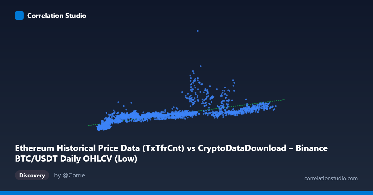
Ethereum Historical Price Data (TxTfrCnt) vs CryptoDataDownload – Binance BTC/USDT Daily OHLCV (Low)
- Pearson correlation (r)
- 0.7554
- Spearman correlation
- 0.9034
- p-value
- 0
- Sample size (n)
- 3191
- 95% confidence interval
- 0.7401 to 0.7699
- Granger causality
- None
- Granger optimal lag
- 10
AI analysis
Analysis: Ethereum Transfer Count vs. BTC/USDT Price Relationship
1. Overview of the Relationship
Despite the confusing axis labels (the metadata suggests mismatched column descriptions), the data show a moderate-to-strong positive association between the X variable (ranging ~2,800–123,000) and Y variable (ranging ~189K–5.25M). As X increases, Y tends to increase as well, but with substantial scatter — this is not a tight, deterministic relationship. The sample points confirm a generally upward trend: low-X values (3,000–10,000) cluster with Y values mostly under 700,000, while higher-X values (60,000–110,000) associate with Y values often exceeding 1,000,000, though with notable exceptions.
2. Strength, Direction, and Statistical Confidence
The Pearson correlation of r = 0.7554 indicates a fairly strong positive linear relationship, but r² = 0.5706 means only 57% of the variance in Y is explained by X — leaving nearly 43% attributable to other factors, noise, or nonlinear dynamics. The 95% CI [0.740, 0.770] is tight, and with n=3,191 and p≈0, we can be highly confident the true population correlation is non-zero and reasonably strong — this is not a spurious finding. However, statistical significance here reflects sample size more than practical predictive power; r² of 0.57 leaves considerable room for large deviations from any fitted line.
Critically, the Granger causality tests show no significant predictive direction in either direction (X→Y: p=0.52; Y→X: p=0.57) at the optimal lag of 10 periods. This means neither variable's past values help forecast the other's future values in a time-series sense. The contemporaneous correlation is real, but it does not imply temporal lead-lag causality — both series likely respond to a shared external driver (e.g., overall market conditions, or in the case of crypto, broad bull/bear cycles) rather than one causing the other.
3. Notable Patterns and Non-linearity
Several features stand out in the sample data: - Outliers/high-leverage points: (65712, 2698591) and (80731, 1847022) and (63888, 1815531) and (89314, 1819052) show Y values 2-3x higher than the general trend line would predict for their X values — these likely correspond to speculative price spikes (bubble periods) decoupled from the X metric. - Compression at low X: Many points with X < 10,000 show Y values spanning 200,000 to 950,000 — a wide range for a narrow X band, suggesting heteroscedasticity (increasing variance at lower X, or a curve that's steep initially). - The note about Spearman ρ exceeding Pearson r is important: this signals rank-order relationship is stronger than the linear one, supporting a logarithmic or power-law fit rather than the linear model shown (y = 9.98x + 450,933). Crypto price/volume relationships are classically log-normal, so a log-log regression would likely fit substantially better and reduce the appearance of "outliers."
4. Confounding Factors and Caveats
Several caveats limit causal interpretation: - Metadata inconsistency: The column descriptions reference overlapping/conflicting datasets (Ethereum TxTfrCnt vs. BTC/USDT OHLCV Low) — it's unclear if X and Y are truly independent metrics or both derivatives of BTC price data. This should be resolved before drawing conclusions. - Shared macro-driver: Both crypto price and on-chain activity metrics (transfer counts) are driven by common market sentiment, Bitcoin dominance cycles, and macroeconomic liquidity conditions (2017–2026 spans multiple bull/bear cycles). This is a classic confounding scenario producing correlation without direct causation. - Non-stationarity: Crypto price series are typically non-stationary (trending), which can inflate correlation coefficients artificially. The Granger test likely differenced the data, which is why it found no relationship despite the strong raw correlation — this discrepancy itself is a red flag for spurious correlation from co-trending series.
5. Actionable Recommendations
1. Refit with log transformation: Given the Spearman/Pearson gap and crypto's typical log-normal distribution, re-run regression as log(Y) ~ log(X) or log(Y) ~ X to capture the likely power-law relationship and improve r². 2. Test stationarity and cointegration: Since Granger causality found nothing but raw correlation is high, run Augmented Dickey-Fuller tests and a cointegration test (Engle-Granger/Johansen) — the variables may be cointegrated even without lead-lag Granger causality, which would be the more appropriate long-run relationship model for trending price data. 3. Segment by market regime: Split data into bull/bear/sideways periods (2017-2018 boom, 2020-2021 bull run, 2022 crash, etc.) and re-examine correlation within regimes to check if the relationship is stable or regime-dependent. 4. Clarify data provenance: Resolve the axis metadata conflict to confirm what X and Y actually represent before using this relationship for any trading or forecasting model. 5. Investigate high-Y outliers: The points with Y 1.8M at moderate X values warrant a timestamp check — they may correspond to specific known price-spike events (e.g., 2021 bull peaks) that should be understood as regime shifts rather than noise.
X dataset: CryptoDataDownload – Binance BTC/USDT Daily OHLCV
Y dataset: Ethereum Historical Price Data
Part of experiment: Bitcoin - CryptoDataDownload – Binance BTC/USDT Daily OHLCV vs Ethereum Historical Price Data