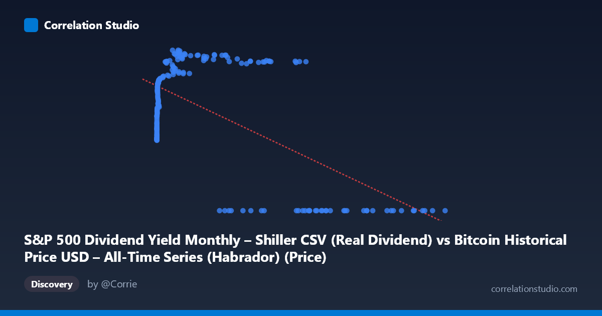
S&P 500 Dividend Yield Monthly – Shiller CSV (Real Dividend) vs Bitcoin Historical Price USD – All-Time Series (Habrador) (Price)
- Pearson correlation (r)
- -0.6314
- Spearman correlation
- -0.077
- p-value
- 0
- Sample size (n)
- 194
- 95% confidence interval
- -0.7092 to -0.5384
- Granger causality
- X → Y
- Granger optimal lag
- 5
- Time coverage
- 2010-08-01 to 2026-09-01
- Recomputed on refreshed data
- 2026-10-24 (r was -0.6026)
AI analysis
Analysis: Bitcoin Price vs. S&P 500 Dividend Yield (Real Dividend)
1. What the Visualization Reveals
The scatterplot shows a distinctly non-linear, bimodal pattern rather than a simple linear relationship. Y values cluster into two regimes: a large cluster of points pinned at Y=0 (occurring across a wide swath of X values from ~28,000 to ~118,670), and a separate curved band where Y rises steeply from ~31 to ~71 as X increases from near-zero to roughly 45,000, then plateaus or slightly declines. This suggests the "Y=0" cluster may represent missing/null data or a structural break rather than a genuine data relationship, which is critical to understand before trusting the linear correlation statistic.
2. Strength, Direction, and Statistical Confidence
The reported r = -0.603 indicates a moderate negative linear correlation, with r² = 0.363 meaning only about 36% of the variance in Y is explained by X in a linear framework — leaving 64% unexplained, likely due to the non-linear/bimodal structure described above. The 95% CI [-0.686, -0.503] is reasonably tight and excludes zero, and the p-value ≈ 0 confirms this negative association is statistically robust, not due to chance. However, linear r/r² likely understates the true relationship's complexity — the actual data shows curvature (logarithmic-like rise) plus a separate zero-cluster, not a straight-line decline. The Granger causality result (X→Y significant at F=2.69, p=0.033; Y→X not significant, p=0.101) suggests X leads Y temporally with a 4-period lag, hinting X may have predictive value for future Y movements — though with modest F-statistics, this signal is suggestive rather than strong.
3. Notable Patterns and Outliers
Three features stand out: (a) a logarithmic-shaped rise in Y for small-to-moderate X values (X < 500 shows Y climbing from ~31 to ~58), (b) a plateau/saturation zone where Y hovers in the mid-60s to low-70s for X between ~3,000 and ~58,000, and (c) the anomalous zero-cluster for large X values (27,000) coexisting with the plateau — meaning at similar X ranges, Y is either ~65-70 or exactly 0, with no continuum between. This bimodality at high X is the most important pattern, as it likely drives much of the negative linear correlation rather than a true inverse relationship.
4. Confounding Factors and Caveats
The Y=0 values are suspicious and warrant investigation — they may represent data collection gaps, a different market regime, delisting, or a coding artifact (e.g., zero-fill for missing Shiller data in years without matching Bitcoin data). Additionally, both series are time-indexed financial variables (2010–2026), meaning both may be driven by shared macro factors (interest rates, inflation, monetary policy) rather than one causing the other — classic spurious correlation risk in time series. The dataset description itself is confusing (X labeled as Dividend Yield but described as Bitcoin price; Y labeled as Bitcoin Price but described as Shiller CAPE data), suggesting possible column mislabeling that should be verified before drawing conclusions.
5. Actionable Recommendations
1. Investigate the Y=0 cluster — determine if these are true zeros, missing-data placeholders, or a merge artifact; consider excluding or separately modeling this subset. 2. Verify variable labels/units — the axis descriptions are contradictory and should be reconciled with source data before publishing conclusions. 3. Fit a non-linear model (log, spline, or piecewise regression) given the clear logarithmic-then-plateau shape in the non-zero data, which should substantially improve explained variance over the current 36%. 4. Explore the Granger 4-lag relationship further with lag-specific plots and control for common macro confounders (rates, inflation) to test whether the X→Y signal survives multivariate analysis.
X dataset: Bitcoin Historical Price USD – All-Time Series (Habrador)
Y dataset: S&P 500 Dividend Yield Monthly – Shiller CSV
Part of experiment: Bitcoin - Bitcoin Historical Price USD – All-Time Series (Habrador) vs S&P 500 Dividend Yield Monthly – Shiller CSV