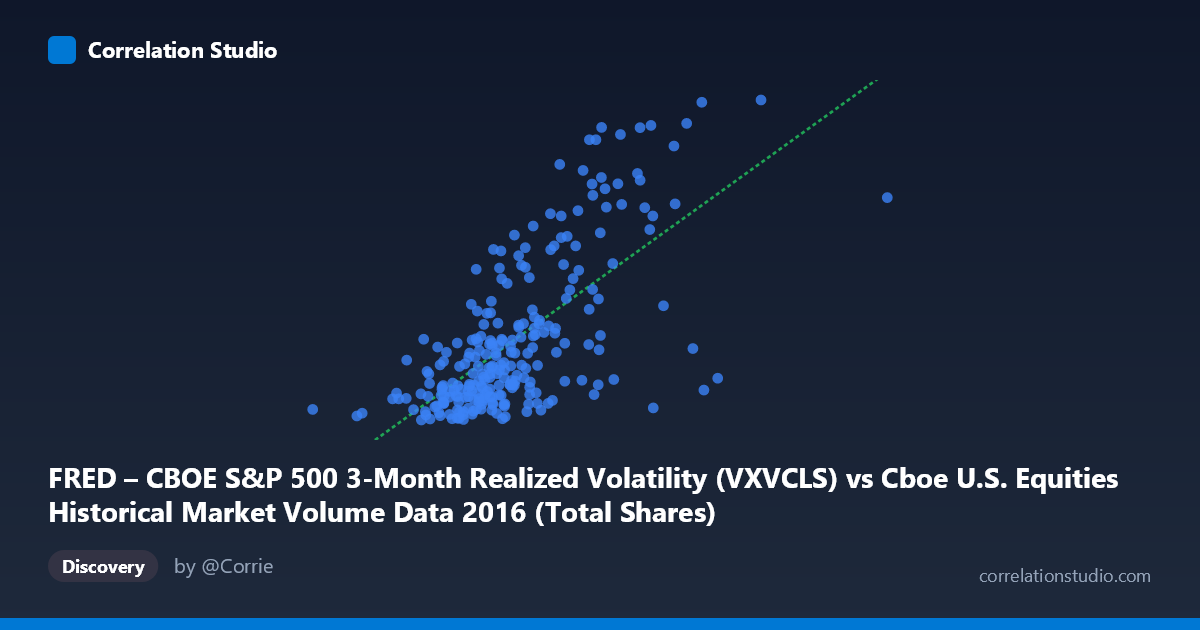
FRED – CBOE S&P 500 3-Month Realized Volatility (VXVCLS) vs Cboe U.S. Equities Historical Market Volume Data 2016 (Total Shares)
- Pearson correlation (r)
- 0.676
- Spearman correlation
- 0.6413
- p-value
- 0
- Sample size (n)
- 252
- 95% confidence interval
- 0.6028 to 0.738
- Granger causality
- None
- Granger optimal lag
- 1
AI analysis
Analysis: CBOE S&P 500 3-Month Realized Volatility vs. U.S. Equities Total Shares Volume (2016)
Relationship Overview The scatterplot reveals a moderate-to-strong positive relationship between CBOE S&P 500 3-month realized volatility (VXVCLS) and total shares traded in U.S. equities markets throughout 2016. As volatility rises, trading volume tends to increase correspondingly — a relationship that is intuitive given that volatile market conditions typically prompt heightened investor activity, both defensive repositioning and opportunistic trading. The linear regression equation (y = 1.84e-08x + 8.83) confirms this positive slope, and the visual distribution of points generally follows this upward trend, though with considerable scatter around the regression line.
Correlation Strength and Statistical Significance The correlation of r = 0.676 indicates a moderately strong positive association, but the more informative metric is r² = 0.457, meaning that roughly 45.7% of the variance in volatility is explained by trading volume (or vice versa). While statistically meaningful, this leaves over half the variance unexplained by this linear relationship alone. The 95% confidence interval of [0.603, 0.738] is relatively tight and does not include zero, reinforcing confidence in the direction and magnitude of the association. With a p-value effectively at zero across a paired sample of n = 252 drawn from a population of N = 3,622, the result is highly statistically significant. However, the Granger causality tests yield no significant directional predictive relationship in either direction (X→Y: F = 0.060, p = 0.807; Y→X: F = 0.576, p = 0.449), meaning that knowing today's volume does not meaningfully help predict tomorrow's volatility, and vice versa. This is a critical caveat: the variables move together contemporaneously but neither reliably leads the other.
Notable Patterns, Clusters, and Outliers Several features stand out in the data. The bulk of observations cluster in a lower-left region — roughly volume below 600M shares and volatility below 20 — suggesting that calm, low-volume trading days dominated much of 2016. However, there are clearly visible high-leverage outliers in the upper-right quadrant, including points near (708M shares, 26.71 vol) and (583M shares, 25.25 vol), which likely correspond to specific market stress events such as the Brexit vote (June 2016) or the U.S. presidential election (November 2016). These extreme observations disproportionately drive the regression slope and correlation coefficient upward. There also appears to be modest heteroscedasticity — the spread of volatility values widens as volume increases — suggesting the linear model may underfit the high-volume regime.
Confounding Factors and Caveats Several important caveats limit causal interpretation. First, both variables are likely driven by common exogenous shocks — macro events, geopolitical surprises, or Fed announcements — making it difficult to attribute directional causation to either series. Second, the axes appear swapped in labeling (X-axis label references VXVCLS but describes volume data, and vice versa), which warrants careful verification before drawing conclusions. Third, the 3-month realized volatility index is a backward-looking measure that smooths over a 63-trading-day window, meaning it may lag the instantaneous market stress that spikes volume on a given day — this structural mismatch could suppress Granger causality even when a true economic relationship exists. Finally, 2016 was an unusual year with discrete, clustered shock events (Brexit, U.S. election), which may inflate the correlation relative to a more typical year.
Actionable Insights and Further Investigation Practitioners monitoring market microstructure conditions should treat elevated realized volatility as a contemporaneous signal of increased volume and liquidity demand, though not a reliable leading indicator for positioning purposes. To deepen this analysis, it would be valuable to: (1) decompose the data by event windows (e.g., Brexit week, election week vs. ordinary days) to assess whether the correlation is event-driven or structural; (2) test nonlinear specifications (e.g., log-log regression) given the apparent heteroscedasticity; (3) extend the time series beyond 2016 to assess whether this r ≈ 0.68 relationship is stable across different volatility regimes; and (4) introduce intraday data or lagged variables at shorter horizons (hours rather than days) where Granger causality may be detectable. The ~54% unexplained variance also invites incorporation of additional predictors such as options market open interest, institutional order flow, or VIX term structure slope.
X dataset: Cboe U.S. Equities Historical Market Volume Data 2016
Y dataset: FRED – CBOE S&P 500 3-Month Realized Volatility
Part of experiment: Daily - Cboe U.S. Equities Historical Market Volume Data 2016 vs FRED – CBOE S&P 500 3-Month Realized Volatility