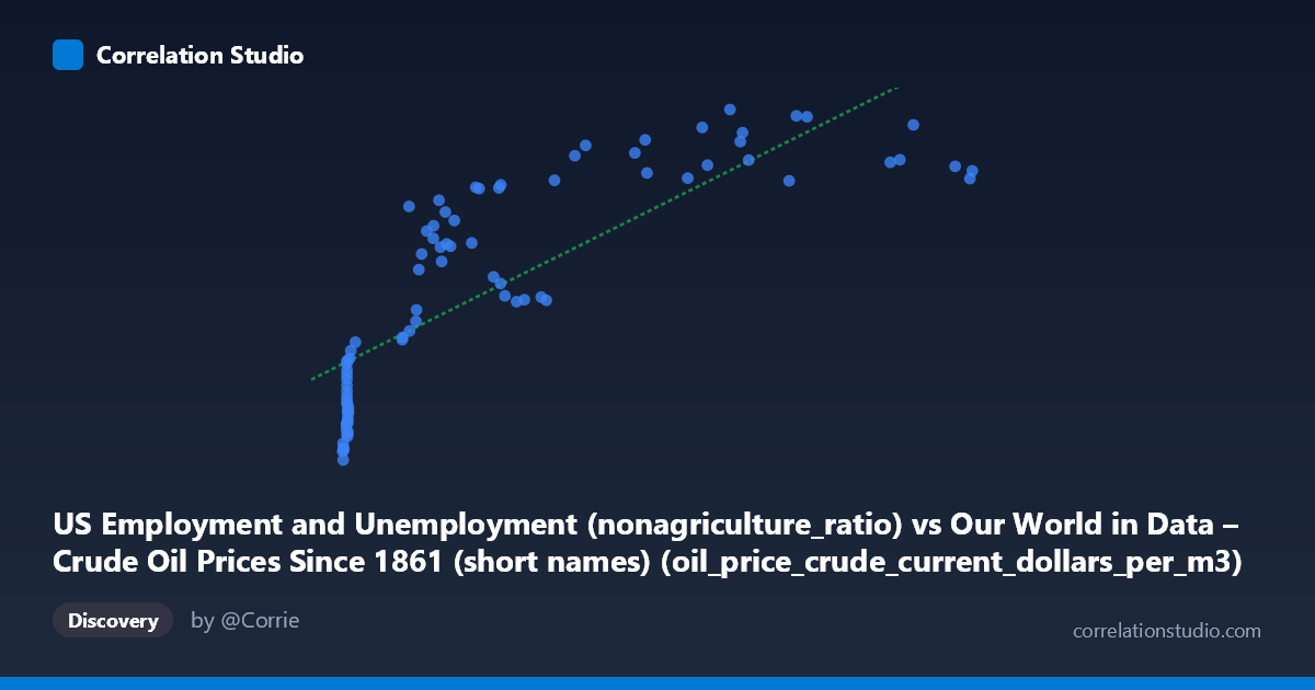
US Employment and Unemployment (nonagriculture_ratio) vs Our World in Data – Crude Oil Prices Since 1861 (short names) (oil_price_crude_current_dollars_per_m3)
- Pearson correlation (r)
- 0.8114
- Spearman correlation
- 0.9157
- p-value
- 0
- Sample size (n)
- 85
- 95% confidence interval
- 0.7233 to 0.8735
- Granger causality
- None
- Granger optimal lag
- 10
AI analysis
Scatterplot Analysis: Non-Agricultural Employment Ratio vs. Crude Oil Prices
1. Visual Relationship Overview
The scatterplot reveals a broadly positive relationship between the US non-agricultural employment ratio and crude oil prices (in current dollars per cubic meter), consistent with the reported Pearson r of 0.807. However, the relationship is clearly not linear throughout its range. At lower X values (roughly 6–150), there is considerable vertical spread, with oil prices ranging from ~$41,000 to over $130,000 per m³ for similar employment ratios. At higher X values (150–700+), the data fans out horizontally while Y values plateau and even begin to decline at the extreme right tail, suggesting a logarithmic or diminishing-returns curve rather than a straight line. This visual impression is reinforced by the note that Spearman ρ exceeds Pearson r, confirming meaningful non-linearity.
2. Correlation Strength, Direction, and Causality
The Pearson r of 0.807 indicates a strong positive correlation, and r² = 0.651 means that approximately 65% of the variance in crude oil prices is statistically explained by variation in the non-agricultural employment ratio — a substantial but incomplete share, leaving 35% attributable to other factors. The 95% confidence interval of [0.716, 0.871] is relatively narrow given the sample size of n=84, and the p-value of effectively zero confirms this association is not a sampling artifact. That said, the Granger causality tests are decidedly non-significant in both directions (X→Y: F=1.12, p=0.364; Y→X: F=1.43, p=0.195), meaning neither variable demonstrably temporally predicts the other after accounting for their own lagged values at the optimal 10-period lag. This is a critical caveat: correlation here reflects co-movement over time, not a predictive or causal mechanism in either direction.
3. Notable Patterns, Clusters, and Outliers
Several structural features stand out:
- Dense low-X cluster: A large concentration of points sits near X = 7–15 (low employment ratio values, likely corresponding to early decades in the dataset, 1940s–1960s), with oil prices in the $41,000–$80,000 range. These points form a near-vertical cluster, showing high variance in Y for minimal variance in X. - Mid-range scatter (X = 70–200): A broad, dispersed cloud with oil prices spanning $80,000–$135,000, suggesting this region of the employment ratio has the weakest predictive power. - High-X plateau and reversal: Above X ≈ 400, oil prices cluster between $136,000–$159,000 but show no continued upward trend, and a few points near X = 700 actually have lower oil prices (~$137,000–$141,000), hinting at a peak or saturation effect. - Potential outliers: Points such as (507.96, 159,091) and (519.80, 158,772) sit at the upper-right boundary and may represent the early 2020s oil price spike, while (699.78, 137,615) and (702.38, 140,283) suggest that extreme employment ratios do not sustain the highest prices.
4. Confounding Factors and Interpretive Caveats
The most important caveat is that both variables are strongly driven by time — as decades progress, both the non-agricultural employment ratio and nominal crude oil prices have generally trended upward, making this correlation substantially a spurious time-trend relationship rather than a structural economic mechanism. Nominal oil prices, in particular, are subject to inflation, OPEC supply decisions, geopolitical shocks (e.g., 1973, 1979, 2008, 2020), and technological change in energy production — none of which are captured by an employment ratio. The employment ratio itself reflects long-run structural shifts in the US labor market (post-WWII industrialization, female labor force participation, deindustrialization) that are only loosely connected to oil markets. The failure of Granger causality in both directions underscores that no reliable temporal predictive pathway exists between these variables. Additionally, the linear regression model (y = 153x + 73,188) is likely misspecified given the visual and statistical evidence of non-linearity.
5. Actionable Insights and Further Investigation
| Recommendation | Rationale | |---|---| | Fit a logarithmic or polynomial regression | Spearman ρ Pearson r; visual plateau at high X values | | Deflate oil prices to real terms | Removes inflation as a dominant confounder masking the true relationship | | Include time as an explicit covariate | Isolates shared time-trend from genuine structural association | | Test sub-period stability | Pre/post-1973 oil shock, pre/post-2000 shale revolution may reveal structurally different regimes | | Introduce intermediate variables | GDP growth, industrial output, and energy intensity could mediate or explain the co-movement |
In summary, while the statistical correlation is strong and significant, the absence of Granger causality in either direction, the evident non-linearity, and the likely confounding role of shared long-run time trends suggest this relationship is descriptive of co-evolution over decades rather than actionable as a predictive or causal model. Any policy or forecasting use of this association would require substantially more robust causal identification.
X dataset: Our World in Data – Crude Oil Prices Since 1861 (short names)
Y dataset: US Employment and Unemployment
Part of experiment: Yearly - Our World in Data – Crude Oil Prices Since 1861 (short names) vs US Employment and Unemployment