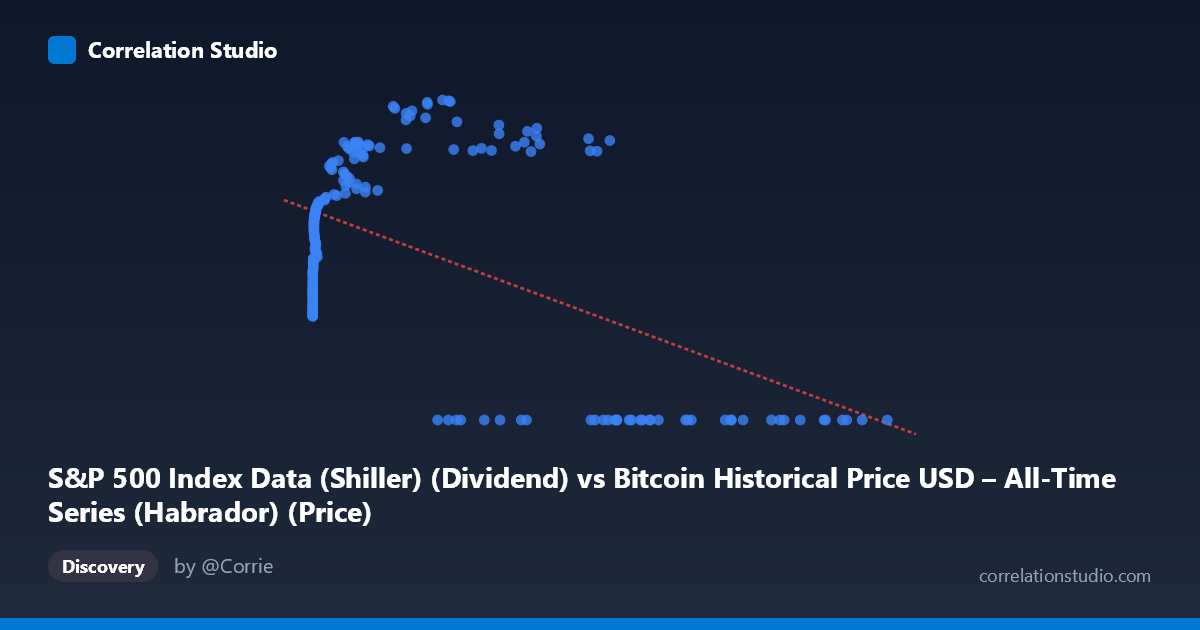
S&P 500 Index Data (Shiller) (Dividend) vs Bitcoin Historical Price USD – All-Time Series (Habrador) (Price)
- Pearson correlation (r)
- -0.5041
- Spearman correlation
- 0.036
- p-value
- 0
- Sample size (n)
- 189
- 95% confidence interval
- -0.6034 to -0.3894
- Granger causality
- X → Y
- Granger optimal lag
- 4
AI analysis
Analysis: Bitcoin Price vs. S&P 500 Index Data
1. What the Visualization Reveals
The scatterplot shows a distinctly non-linear, non-monotonic relationship rather than a simple linear correlation. At low X values (roughly 0–2,000), Y rises steeply from ~22 to ~50-55 as X increases—a clear positive relationship. Then, in a middle range (X ≈ 3,000–60,000), Y continues climbing modestly and plateaus in the upper 50s-60s. But at high X values (60,000), Y collapses abruptly to 0 in nearly every case. This creates a pattern that looks less like a continuous trend and more like two regimes: a rising curve at low-to-mid X, and a hard floor of zero at high X. The reported linear correlation (r = -0.504) is essentially an artifact of this bifurcated structure—the cluster of high-X/zero-Y points pulls the linear fit downward, masking the actual positive relationship that dominates most of the data range.
2. Strength, Direction, and Statistical Confidence
The linear r² of 0.254 indicates the straight-line model explains only about 25% of variance in Y — a weak-to-moderate fit that is a poor description of the true (curved) relationship visible in the chart. The negative sign is driven almost entirely by the zero-Y cluster at extreme X values, not by a genuine inverse relationship in the bulk of the data. The 95% CI [-0.603, -0.389] is fairly tight and excludes zero, and the p-value (1.4e-13) confirms the linear correlation is statistically robust — but "statistically significant" here does not mean "correctly specified." A quadratic or piecewise/threshold model would likely fit dramatically better than r²=0.25.
The Granger causality result (X→Y significant at lag 4, p=0.029; Y→X not significant, p=0.116) suggests X's history has some predictive content for Y beyond Y's own history, at a 4-period lag. This is modest evidence (p is close to 0.05, F=2.76) and should be treated cautiously — it indicates temporal precedence/predictability, not proven causation, especially given the non-linear, regime-like structure that likely violates the linear assumptions underlying Granger tests.
3. Notable Patterns, Clusters, and Outliers
Three visible clusters stand out: - Low-X cluster (X < 20): tight grouping with Y in low-to-mid 20s — likely early Bitcoin history when prices were near-zero. - Rising-curve cluster (X: 100–60,000): Y climbs from ~33 to ~68, suggesting a genuine positive co-movement phase. - Zero-Y cluster (X 27,000, especially 60,000): numerous points with Y exactly 0.00, an unusual concentration that looks like a data artifact, missing-value placeholder, or a structural break (e.g., dividend/index data unavailable or reported as zero for certain periods) rather than a true observed value.
This zero-cluster is the single most influential feature in the dataset and warrants specific investigation — it may be driving both the negative linear r and the apparent "high-X" behavior.
4. Confounding Factors and Caveats
Several concerns limit causal interpretation: - Non-stationarity: Both Bitcoin price and S&P 500-derived series exhibit strong trends/growth over time; correlations between two trending series are often spurious unless differenced or detrended. - Time coverage mismatch: The 2010–2026 window spans vastly different Bitcoin market regimes (early speculative years vs. institutional adoption), and macro conditions (rates, inflation, dividend policy) affecting the S&P side changed too. - Zero-value artifact: The Y=0 cluster at high X looks suspicious — possibly missing/placeholder data rather than genuine index values, which would artificially inflate the negative correlation and distort both regression and Granger results. - Sample size: n=189 paired points from a population of 1,865 — the subsampling method could introduce selection bias, especially if not random.
5. Actionable Insights
Before drawing causal conclusions, (a) investigate and likely exclude/impute the Y=0 data points to determine if they represent genuine values or missing data; (b) refit using a non-linear model (polynomial, spline, or piecewise regression) given the visibly curved relationship, and compare against the linear r²=0.25 baseline; (c) apply differencing or log-transforms to address non-stationarity before re-running Granger causality, since trending series can produce misleading lag-predictive signals; and (d) segment the analysis by Bitcoin market era (early/mid/late) to check whether the relationship is stable or regime-dependent, since a single pooled correlation likely obscures meaningfully different dynamics across time periods.
X dataset: Bitcoin Historical Price USD – All-Time Series (Habrador)
Y dataset: S&P 500 Index Data (Shiller)
Part of experiment: Bitcoin - Bitcoin Historical Price USD – All-Time Series (Habrador) vs S&P 500 Index Data (Shiller)