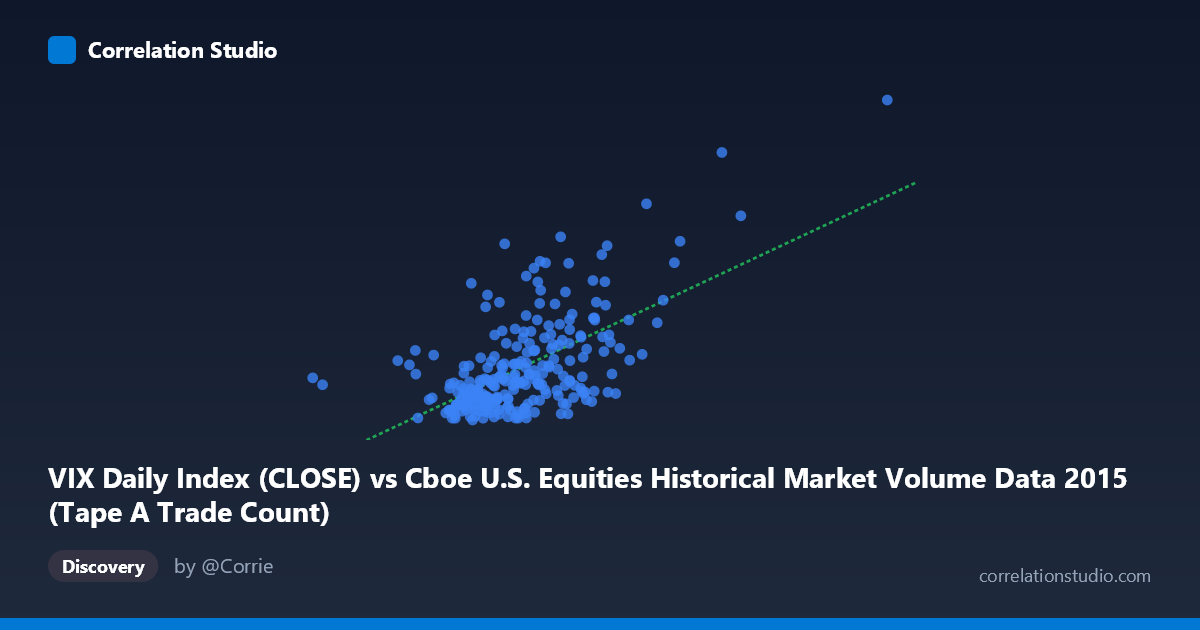
VIX Daily Index (CLOSE) vs Cboe U.S. Equities Historical Market Volume Data 2015 (Tape A Trade Count)

Pearson correlation (r): 0.6064
Spearman correlation: 0.5158
p-value: 0
Sample size (n): 252
95% confidence interval: 0.522 to 0.6791
Granger causality: None
Granger optimal lag: 1

AI analysis

Scatterplot Analysis: VIX Daily Index vs. Tape A Trade Count (2015)

Relationship Overview The scatterplot reveals a positive relationship between the CBOE Volatility Index (VIX) close values and Tape A trade counts across U.S. equity exchanges in 2015. As VIX levels rise — indicating greater market fear or uncertainty — trading activity (measured by trade count) tends to increase correspondingly. This is an intuitively logical pairing: heightened volatility typically triggers more frequent portfolio rebalancing, hedging activity, and speculative trading, all of which drive up transaction volumes. The linear regression equation (y = 1.03×10⁻⁵x + 1.921) confirms a positive slope, though the intercept and scale differences between variables deserve careful interpretation.

Correlation Strength and Statistical Significance The Pearson correlation of r = 0.606 indicates a moderate-to-strong positive association, but the explanatory power is more sobering: r² = 0.368 means only 36.8% of variance in trade count is explained by VIX levels, leaving nearly two-thirds attributable to other factors. The 95% confidence interval of [0.522, 0.679] is reassuringly narrow given the sample size (n = 252), and the p-value of effectively zero confirms this is not a chance result. However, the Granger causality tests tell a critical story: neither direction (X→Y: F=0.244, p=0.622; Y→X: F=0.212, p=0.646) achieves significance. This means that despite the contemporaneous correlation, VIX does not reliably predict future trade counts, nor vice versa — the relationship appears coincident rather than directionally predictive at a one-period lag.

Notable Patterns and Outliers Several features stand out in the sample data. There is a dense cluster of observations in the lower-left region (VIX roughly 576K–1.5M range, trade counts 11–17), suggesting that during periods of normal or low volatility, trade activity remains relatively compressed and homogeneous. However, at higher VIX levels, the data fans outward considerably, suggesting heteroscedasticity — variance in trade count increases as VIX rises. Notable outliers include the point near (2,247,816, 36.02) and (2,076,907, 28.03), which correspond to extreme volatility episodes likely associated with the August 2015 market correction. The point at (576,208, 15.74) represents an unusually low VIX observation that sits somewhat isolated from the main cluster, potentially a low-volume holiday or anomalous session.

Confounding Factors and Caveats Several important caveats apply. First, the axis labels appear swapped relative to conventional usage — VIX is listed as the X-axis variable but sourced from the "Market Volume" dataset, and trade count is on Y but sourced from the "VIX" dataset, suggesting possible data labeling or merging errors that warrant verification before drawing firm conclusions. Second, seasonality is a significant confounder: both VIX and trade volumes follow cyclical patterns within a calendar year (2015), and their co-movement may partly reflect shared seasonal drivers rather than a direct mechanism. Third, regime shifts like the August 2015 flash crash create structural breaks that disproportionately inflate the correlation. Fourth, the N=3,302 population versus n=252 sample raises questions about whether sampling was truly random or time-sequential, which affects the independence assumption underlying the correlation test.

Actionable Insights and Further Investigation Practitioners could explore rolling-window correlations across sub-periods of 2015 to assess whether the relationship strengthens specifically during high-volatility regimes (e.g., August–September) versus calm periods. Given the Granger causality null result, trading strategies based on using VIX to predict next-day volume (or vice versa) are not supported by this data alone — though longer lag structures (beyond one period) should be tested. Incorporating additional variables such as options volume, bid-ask spreads, or macro news event indicators could help explain the remaining 63% of variance. A quantile regression or log-transformation of VIX values may better capture the non-linear, heteroscedastic structure visible at the high end of the distribution. Finally, replicating this analysis across multiple years would help distinguish structural relationships from 2015-specific dynamics like the China-driven volatility spike.

X dataset: Cboe U.S. Equities Historical Market Volume Data 2015

Y dataset: VIX Daily Index

Part of experiment: Daily - Cboe U.S. Equities Historical Market Volume Data 2015 vs VIX Daily Index