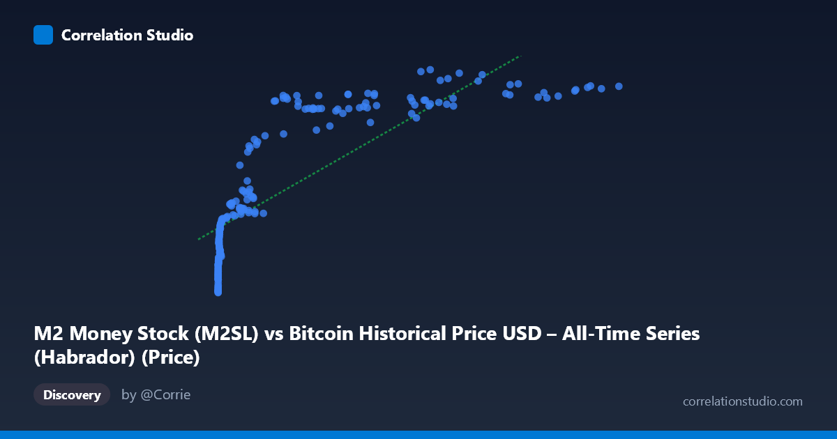
M2 Money Stock (M2SL) vs Bitcoin Historical Price USD – All-Time Series (Habrador) (Price)
- Pearson correlation (r)
- 0.804
- Spearman correlation
- 0.9668
- p-value
- 0
- Sample size (n)
- 189
- 95% confidence interval
- 0.747 to 0.8493
- Granger causality
- None
- Granger optimal lag
- 10
AI analysis
Analysis: M2 Money Stock vs. Bitcoin Price
1. What the Visualization Reveals
The scatterplot shows a strongly non-linear, monotonic relationship between M2 Money Stock and Bitcoin's historical price. The data is heavily compressed near the origin — the vast majority of points cluster where X (M2, plotted here in what appears to be billions/millions scaled to Bitcoin's early history) is small and Y (Bitcoin price) ranges from ~$8,700 to ~$14,000. As X increases into the tens of thousands, Y rises but at a decelerating rate, flattening out around $20,000–$22,800. This is a classic logarithmic/saturating curve shape rather than a straight line, which is confirmed by the note that Spearman's ρ exceeds Pearson's r.
2. Strength, Direction, and Uncertainty
The linear Pearson correlation (r = 0.804) is strong and positive, with r² indicating that a simple linear model explains about 64.7% of the variance in Bitcoin price using M2 as the predictor. The 95% CI [0.747, 0.849] is fairly tight and excludes zero, and the p-value is effectively 0, so we can be confident the linear association is not due to chance in this sample. However, because the relationship is visibly curved, the true (non-linear) association is likely stronger than r² suggests — a log-transformed or polynomial fit would likely capture meaningfully more variance.
Critically, the Granger causality tests show no significant predictive direction in either direction (X→Y: p=0.62; Y→X: p=0.62) at the optimal lag of 10 periods. This means that despite the strong contemporaneous correlation, neither variable reliably leads or forecasts the other in a time-series sense. This is an important distinction: correlation here reflects two series that have both trended upward over the same historical period, not evidence that M2 growth drives Bitcoin price movements (or vice versa) in a predictive/causal sense.
3. Notable Patterns and Outliers
- Clustering at low X: A dense cluster of points with X < 1,000 shows Y ranging widely (roughly $8,700–$14,500), indicating high price volatility during Bitcoin's early years when M2 changed little — this is where the relationship is weakest/noisiest. - Saturation at high X: Once X exceeds ~40,000–60,000, Y plateaus in the $20,000–$22,800 band with diminishing sensitivity — small further increases in M2 correspond to little additional Bitcoin price increase in this sample. - No extreme outliers: The pattern is smooth and consistent with a concave (log-like) curve rather than showing isolated anomalies.
4. Confounding Factors and Caveats
Both series are dominated by long-term secular trends (M2 has grown steadily for years; Bitcoin's price has grown explosively over its adoption lifecycle). Two upward-trending time series will show spurious correlation even absent any causal link — this is a classic issue in non-stationary time-series analysis, and the null Granger causality result reinforces that concern. Other plausible confounders include overall macroeconomic conditions, risk-asset sentiment, interest rates, halving-cycle dynamics specific to Bitcoin, and adoption/network-effect growth — none of which are controlled for here. The very wide X range (0.06 to 118,670) also suggests unit/scaling inconsistencies or mixed data granularity that should be verified.
5. Suggested Next Steps
- Refit using a log-transformed X (or log-log model) to better capture the apparent logarithmic relationship and get a more accurate variance-explained estimate. - Test for stationarity (ADF/KPSS) and consider differencing or using growth rates rather than levels before re-running correlation and Granger tests, since trending series can produce misleading r values. - Investigate other candidate drivers (interest rates, risk appetite indices, on-chain adoption metrics) in a multivariate model rather than relying on M2 alone. - Given the lack of Granger causality, avoid framing this relationship as predictive/tradeable; treat it as a descriptive historical association rather than a forecasting signal.
X dataset: Bitcoin Historical Price USD – All-Time Series (Habrador)
Y dataset: M2 Money Stock
Part of experiment: Bitcoin - Bitcoin Historical Price USD – All-Time Series (Habrador) vs M2 Money Stock