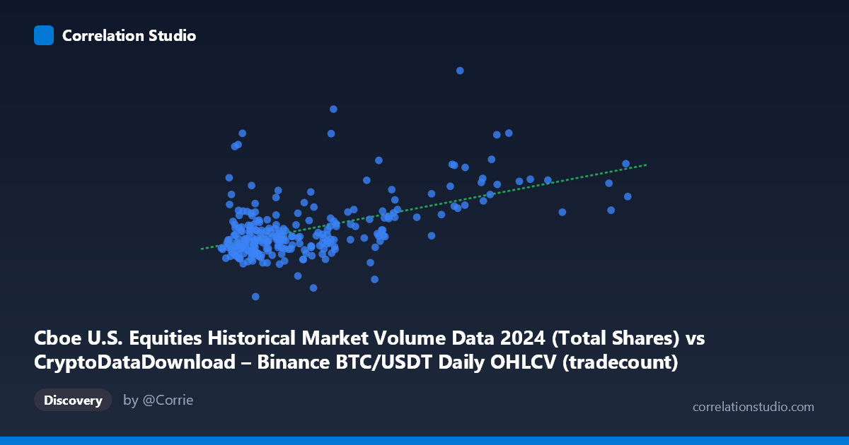
Cboe U.S. Equities Historical Market Volume Data 2024 (Total Shares) vs CryptoDataDownload – Binance BTC/USDT Daily OHLCV (tradecount)
- Pearson correlation (r)
- 0.5209
- Spearman correlation
- 0.3932
- p-value
- 0
- Sample size (n)
- 252
- 95% confidence interval
- 0.4246 to 0.6055
- Granger causality
- None
- Granger optimal lag
- 10
AI analysis
Analysis: Cboe Equities Volume vs. Binance BTC/USDT Trade Count
1. Relationship Overview
The scatterplot shows a moderate positive relationship between the two variables: as one metric (X) increases, the other (Y) tends to increase as well, though with substantial scatter. The data is heavily concentrated in a lower range of X values (roughly 900,000–5,000,000), with a sparser tail of higher-X observations (5,000,000–12,000,000) that appear to pull the trend upward. This clustering pattern suggests the relationship may not be uniformly linear across the full range of X.
2. Strength, Direction, and Statistical Confidence
The correlation coefficient (r = 0.52) indicates a moderate positive association, with r² = 0.271 meaning only 27% of the variance in Y is explained by X — leaving roughly 73% attributable to other factors, noise, or nonlinear dynamics. The 95% confidence interval [0.42, 0.61] is reasonably tight and excludes zero, and the p-value (effectively 0) confirms this correlation is highly unlikely to be due to chance at n=252. However, statistical significance here reflects sample size more than practical predictive power — r² of 0.27 is a weak-to-moderate explanatory relationship, not one suited for precise forecasting.
Critically, the Granger causality tests show no significant predictive direction in either direction (X→Y: p=0.64; Y→X: p=0.58) even at an optimal lag of 10 periods. This means neither series meaningfully helps predict future values of the other over time — the correlation is likely contemporaneous/coincidental rather than causal or lead-lag in nature. This is an important distinction: two variables can be correlated in cross-section while having no temporal forecasting relationship.
3. Patterns, Clusters, and Outliers
The data shows a dense cluster of points where X is low (under 3,000,000) and Y ranges widely (380M–970M), suggesting high Y-variability that's poorly explained by X in this region. A secondary cluster with higher X (5,000,000–9,000,000) also shows elevated Y values (700M–880M), which may be driving much of the apparent linear trend. Notable outliers include the point at (1,362,617, 965,858,507) — unusually high Y for a low X value — and (1,839,372, 379,683,190), which is the minimum Y value paired with a low-to-mid X. These outliers, along with the gap in X between ~5.6M and ~7.5M, suggest the "trend" may partly be an artifact of sparse sampling in the mid-to-upper X range rather than a smooth continuous relationship.
4. Confounding Factors and Caveats
Several caveats are essential here: - Mismatched entities: This compares BTC/USDT trade counts (crypto) against U.S. equities market volume (Cboe) — two unrelated market structures. Any correlation is likely driven by a shared external driver (e.g., overall market-wide volatility, macroeconomic news cycles, or seasonal trading patterns in 2024) rather than a direct mechanistic link. - Time aggregation: Both series are daily 2024 data; common calendar effects (weekday/weekend patterns, holidays, quarter-end rebalancing) could inflate correlation without genuine economic connection. - Non-stationarity: Financial volume/trade-count series often trend or exhibit volatility clustering; if both series trended over 2024 independently, this alone can generate spurious correlation. - Sample vs. population: n=252 sampled from N=3,212 — worth verifying the sampling method preserved time-series structure, especially given the Granger test's temporal assumptions.
5. Recommendations for Further Investigation
- Test for spurious correlation: Run stationarity tests (ADF/KPSS) on both series; if non-stationary, consider differencing or examining cointegration rather than raw-level correlation. - Identify shared confounders: Introduce a third variable (e.g., VIX, overall crypto market cap, or macro news events) to test whether it explains the co-movement better than a direct link. - Segment the analysis: Given the clustering pattern, consider whether splitting data into "low-X" and "high-X" regimes reveals different (possibly stronger or weaker) relationships in each subset. - Given the null Granger result, avoid using either series as a leading indicator for the other in forecasting models — treat this as a same-day associative relationship only, not a predictive one.
X dataset: CryptoDataDownload – Binance BTC/USDT Daily OHLCV
Y dataset: Cboe U.S. Equities Historical Market Volume Data 2024
Part of experiment: Bitcoin - CryptoDataDownload – Binance BTC/USDT Daily OHLCV vs Cboe U.S. Equities Historical Market Volume Data 2024