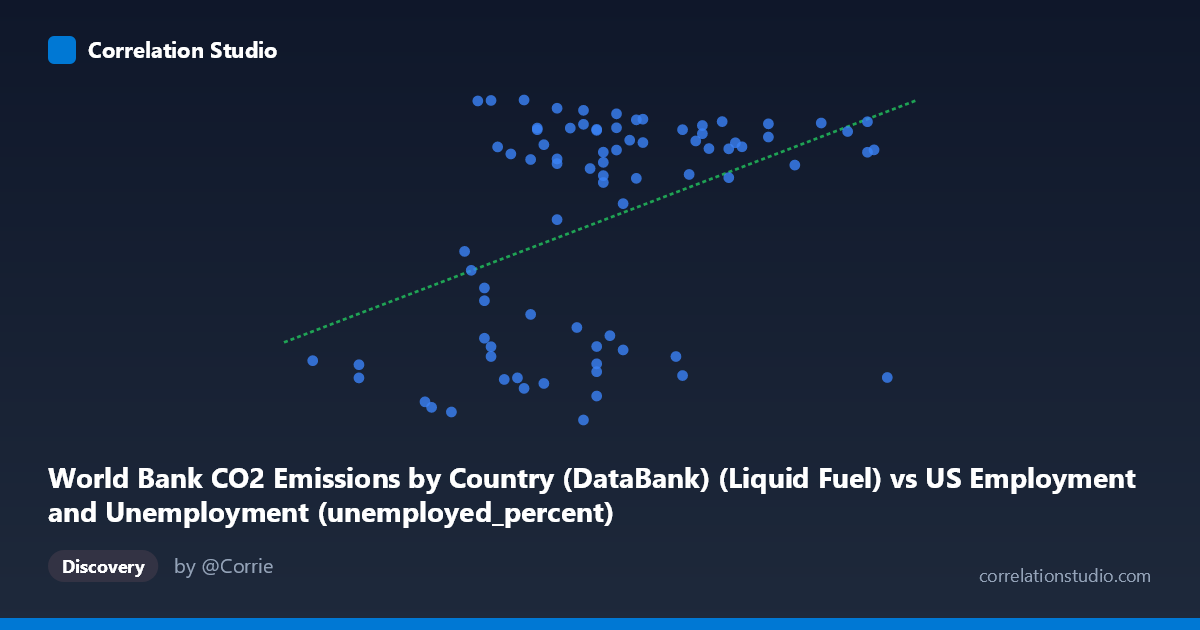
World Bank CO2 Emissions by Country (DataBank) (Liquid Fuel) vs US Employment and Unemployment (unemployed_percent)
- Pearson correlation (r)
- 0.4272
- Spearman correlation
- 0.3747
- p-value
- 0.000078
- Sample size (n)
- 80
- 95% confidence interval
- 0.229 to 0.5914
- Granger causality
- None
- Granger optimal lag
- 10
AI analysis
Scatterplot Analysis: Liquid Fuel CO2 Emissions vs. US Unemployment Rate
1. Overall Relationship
The scatterplot reveals a modest positive relationship between World Bank liquid fuel CO2 emissions and the US unemployment percentage over the period 1941–2020. The linear regression equation (y = 877.13x + 4519.59) suggests that for each unit increase in the liquid fuel CO2 emissions variable, unemployment tends to rise by approximately 877 units. However, the scatter of points around this regression line is substantial, indicating that the linear relationship captures only a fraction of the overall variability in the data. Visually, the cloud of points is wide and diffuse, with no tightly clustered linear band, which immediately signals a weak-to-moderate fit rather than a compelling structural relationship.
2. Correlation Strength, Direction, and Temporal Causality
The Pearson correlation coefficient of r = 0.4272 indicates a weak-to-moderate positive association. More informatively, R² = 0.1825, meaning that liquid fuel CO2 emissions explain only 18.2% of the variance in US unemployment — leaving over 80% of the variation attributable to other factors entirely. While statistically significant (p = 7.75×10⁻⁵, well below the conventional 0.05 threshold), statistical significance here is partly a function of the reasonably large sample size (n = 80) rather than a reflection of a practically strong relationship. The 95% confidence interval for r [0.229, 0.591] is notably wide, spanning from a near-negligible to a moderate correlation, underscoring meaningful uncertainty about the true population effect size. Critically, the Granger causality analysis finds no significant predictive direction in either direction (X→Y: F = 0.47, p = 0.90; Y→X: F = 0.84, p = 0.60), meaning that neither variable temporally predicts the other even at the optimal lag of 10 periods. This effectively rules out any straightforward leading-indicator or causal temporal pathway between these two series.
3. Notable Patterns, Clusters, and Outliers
The scatterplot reveals a striking bimodal or two-cluster structure in the Y-axis (unemployment) values. A dense cluster of points hovers in the ~11,000–13,600 range, while a separate cluster sits at ~2,500–6,500, with relatively few points in the intermediate range (~7,000–10,000). This bimodal distribution strongly suggests that unemployment is not varying continuously and smoothly with CO2 emissions, but rather occupying two distinct regimes — likely corresponding to recessionary versus expansion periods in the US economy. Several potential outliers are visible: the point near (9.90, ~3,972) represents a high-emission observation paired with very low unemployment, which runs counter to the positive trend. Similarly, points near (3.90, ~13,586) and (4.40, ~13,602) show low emissions but very high unemployment values. These outliers pull against the correlation and may correspond to specific historical episodes such as the Great Depression aftermath, wartime mobilization, or the COVID-19 era.
4. Confounding Factors and Caveats
Several important caveats temper any causal interpretation. First, both variables are time-series, and their apparent correlation may be driven by shared secular trends — global CO2 emissions have generally increased over the 20th century while US unemployment fluctuates with business cycles — making spurious correlation a genuine risk. The absence of Granger causality supports this skepticism. Second, the dataset pairing itself is conceptually unusual: liquid fuel CO2 emissions are a global aggregate (World Bank), while unemployment is a US-specific metric, so any link between them is almost certainly mediated by a web of third variables such as global GDP growth, oil price shocks, technological change, and geopolitical events. Third, the bimodal Y distribution violates the homoscedasticity assumption underlying linear regression, suggesting the linear model is likely misspecified and that a simple r/R² framework may be misleading. Fourth, the 80-year time span (1941–2020) encompasses radically different economic regimes, wars, energy transitions, and structural labor market shifts that confound any stable cross-period correlation.
5. Actionable Insights and Further Investigation
Given these findings, several analytical directions are warranted. Regime-based segmentation — splitting the data into distinct economic eras (e.g., post-WWII expansion, stagflation 1970s, neoliberal era, post-2008) — could reveal whether the correlation is consistent across periods or an artifact of aggregation. Oil price shocks should be introduced as a mediating variable, since they plausibly affect both fossil fuel consumption and unemployment simultaneously. A non-linear or piecewise regression would better capture the apparent bimodal structure in unemployment outcomes. Researchers should also consider replacing global liquid fuel emissions with US-specific energy consumption data to improve conceptual alignment between the two variables. Finally, a vector autoregression (VAR) model with additional controls (GDP, oil prices, labor force participation) would provide a more rigorous test of any dynamic relationship than the current bivariate Granger framework, and would help isolate whether any observed association is genuinely structural or purely coincidental over this long historical window.
X dataset: US Employment and Unemployment
Y dataset: World Bank CO2 Emissions by Country (DataBank)
Part of experiment: Yearly - US Employment and Unemployment vs World Bank CO2 Emissions by Country (DataBank)