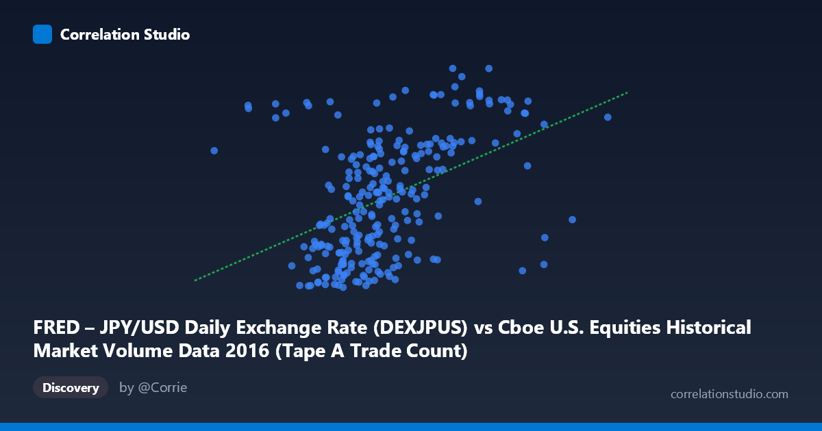
FRED – JPY/USD Daily Exchange Rate (DEXJPUS) vs Cboe U.S. Equities Historical Market Volume Data 2016 (Tape A Trade Count)
- Pearson correlation (r)
- 0.4342
- Spearman correlation
- 0.4859
- p-value
- 0
- Sample size (n)
- 250
- 95% confidence interval
- 0.3278 to 0.5297
- Granger causality
- Y → X
- Granger optimal lag
- 1
AI analysis
Analysis: JPY/USD Exchange Rate vs. Cboe U.S. Equities Trade Count (2016)
Relationship Overview The scatterplot reveals a modest positive relationship between the JPY/USD daily exchange rate (X-axis, representing yen per dollar) and the Cboe U.S. equities Tape A trade count (Y-axis). As the dollar strengthens relative to the yen (higher X values, meaning more yen per dollar), trade counts tend to be somewhat elevated. The linear regression equation (y = 8.38×10⁻⁶x + 97.00) confirms this positive slope, though the scatter is substantial throughout the range, suggesting the relationship is real but far from deterministic. The visualization likely shows a diffuse cloud of points with a gentle upward trend rather than a tight linear band.
Correlation Strength and Statistical Significance The Pearson correlation of r = 0.4342 indicates a moderate positive association, but the explanatory power is limited: R² = 0.1885 means only 18.9% of the variance in trade counts is explained by the exchange rate level. The remaining ~81% is attributable to other factors entirely. The 95% confidence interval [0.328, 0.530] is reasonably tight and does not include zero, and the p-value of 6.44×10⁻¹³ confirms this correlation is highly statistically significant given the large population (N = 3,622). However, statistical significance here is partly a function of sample size — significance does not imply strong practical predictability. Critically, the Granger causality analysis reveals a unidirectional temporal relationship: Y Granger-causes X (F = 5.17, p = 0.024 at lag 1), meaning past trade count levels carry predictive information about future exchange rate movements, but the reverse is not true (F = 0.12, p = 0.729). This inverts the intuitive causal assumption and warrants careful interpretation.
Notable Patterns and Outliers The sample points reveal several notable features. There is a cluster of observations concentrated in the X range of roughly 1,050,000–1,550,000 (the modal range for this exchange rate period), with Y values spanning approximately 100–115 trade count units. A handful of high-X outliers are visible — particularly around X ≈ 2,184,215 (Y = 104.84) and X ≈ 2,321,280 (Y = 106.56) — which represent unusually high exchange rate values but only moderate trade counts, potentially pulling the regression line and weakening the apparent relationship. On the high-Y end, points like (1,726,299, 121.06) and (1,860,056, 118.61) suggest that peak trade counts tend to occur at moderate-to-high exchange rate values, not at the extremes. The presence of low-trade-count days scattered across all X values implies that exchange rate level alone is insufficient to predict market activity.
Confounding Factors and Caveats Several important caveats apply. First, both variables are time series covering the same 2016 calendar year, meaning they share common temporal drivers — volatility events, macro announcements (Fed decisions, Brexit aftermath, U.S. election), and seasonal patterns — that could create spurious correlation. Second, the Granger causality direction (trade count predicting exchange rates) is counterintuitive and may reflect a shared response to unmeasured drivers rather than genuine predictive causality; Granger causality is a statistical, not structural, concept. Third, the X-axis label and Y-axis label appear to be swapped in the dataset metadata (the FRED JPY/USD series is plotted on X but described under Y's dataset, and vice versa), which may indicate a data joining artifact worth verifying. Finally, the exchange rate range spans values from ~540,000 to ~2,497,000, which if interpreted literally as yen-per-dollar would be economically nonsensical (the actual 2016 JPY/USD rate ranged ~100–120), suggesting the X variable may actually represent trade volume or notional value mislabeled, or the axes are indeed inverted.
Actionable Insights and Further Investigation Given the label discrepancy, the first priority should be verifying the correct axis assignments and ensuring the join between the FRED exchange rate series and the Cboe volume data was performed on matching dates without misalignment. If the data is confirmed correct, researchers should investigate whether the correlation strengthens during specific sub-periods (e.g., post-election volatility in Q4 2016), as pooling across regimes may obscure stronger within-regime relationships. The Granger causality finding — that trade activity predicts subsequent exchange rate moves — deserves deeper examination using vector autoregression (VAR) models with additional control variables (VIX, S&P 500 returns, Fed policy dates). Incorporating lagged variables and controlling for day-of-week and macro announcement effects would help isolate whether any genuine predictive signal exists beyond shared temporal structure. An R² of ~19% leaves substantial room for a richer multivariate model.
X dataset: Cboe U.S. Equities Historical Market Volume Data 2016
Y dataset: FRED – JPY/USD Daily Exchange Rate
Part of experiment: Daily - Cboe U.S. Equities Historical Market Volume Data 2016 vs FRED – JPY/USD Daily Exchange Rate