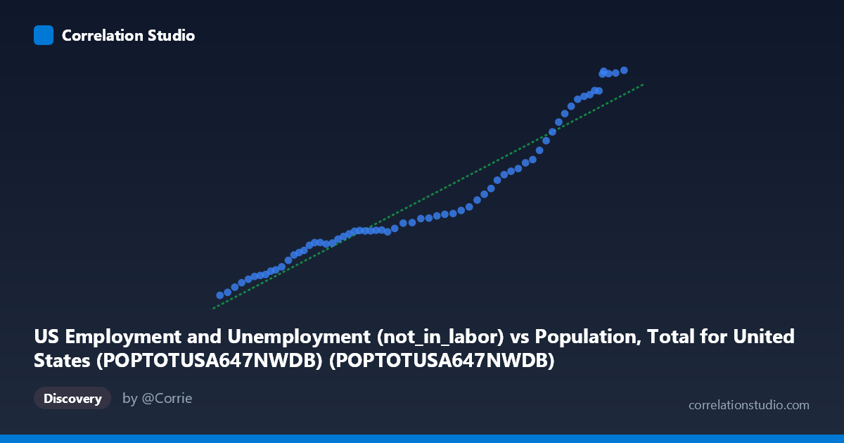
US Employment and Unemployment (not_in_labor) vs Population, Total for United States (POPTOTUSA647NWDB) (POPTOTUSA647NWDB)
- Pearson correlation (r)
- 0.9664
- Spearman correlation
- 0.9984
- p-value
- 0
- Sample size (n)
- 65
- 95% confidence interval
- 0.9453 to 0.9794
- Granger causality
- None
- Granger optimal lag
- 10
AI analysis
Analysis of US Total Population vs. Not-in-Labor-Force
1. What the Visualization Reveals
The scatterplot displays a strong, positive, and largely linear relationship between total US population (X-axis) and the number of Americans not in the labor force (Y-axis) across annual observations from 1960 to 2024. As the population grows from approximately 181 million to 340 million, the not-in-labor-force count rises correspondingly from roughly 47,600 to 100,500 (in thousands). The data points cluster tightly around the regression line y = 0.000310x − 10,671, suggesting a remarkably consistent structural relationship over six decades. Visually, the relationship appears nearly monotonic with little scatter, indicating that population size is a powerful predictor of this labor metric across the full time span.
2. Correlation Strength, Direction, and Causality
The Pearson correlation of r = 0.9664 reflects an exceptionally strong positive association, and the coefficient of determination R² = 0.9339 means that approximately 93.4% of the variance in the not-in-labor-force count is statistically explained by total population size alone. This is a remarkably high explanatory share for a single-variable model. The 95% confidence interval for r of [0.9453, 0.9794] is narrow and excludes zero by a wide margin, while the p-value of ~0 confirms the result is statistically significant far beyond conventional thresholds — the probability of observing this relationship by chance is essentially nil. However, the Granger causality tests reveal no statistically significant predictive direction in either direction (X→Y: F = 1.32, p = 0.26; Y→X: F = 1.28, p = 0.28). This is a critical nuance: despite the overwhelming cross-sectional correlation, neither variable temporally predicts the other beyond what each already contains in its own lagged history. This suggests the two series are co-evolving time trends rather than one driving the other in a causal temporal sense.
3. Notable Patterns, Clusters, and Features
The data points form a single, coherent band with no dramatic breaks or discontinuities, which is consistent with a shared underlying demographic trend. However, closer inspection likely reveals mild clustering in two regions: a lower-left cluster corresponding to the 1960s–1980s (lower population, lower not-in-labor-force counts) and an upper-right cluster for the 2000s–2024 period, particularly where population exceeds ~310 million. Points in the upper range (X 320 million) may show a slightly steeper trajectory, possibly reflecting the aging Baby Boomer cohort entering retirement and exiting the labor force at an accelerating rate — a potential subtle non-linearity at the upper tail. No extreme outliers appear to distort the regression line significantly given the high R².
4. Confounding Factors and Caveats
The most significant interpretive caveat here is spurious correlation driven by shared temporal trends. Both series increase over time as natural functions of demographic growth and societal aging — they are essentially two different measurements of an expanding population. The not-in-labor-force figure mechanically includes retirees, students, homemakers, and discouraged workers, all of which scale broadly with population. This means the strong correlation largely reflects the common trajectory of time rather than a direct structural or causal mechanism between the two specific constructs. Additionally, compositional shifts — such as the Baby Boom cohort aging out of the workforce, rising college enrollment, and changing female labor force participation — alter the relationship over sub-periods in ways the linear model cannot capture. The optimal Granger lag of 10 periods is also quite long, suggesting the test may lack power at shorter, more economically meaningful horizons.
5. Actionable Insights and Further Investigation
Given that the correlation is primarily driven by shared demographic trends, analysts should detrend both series (e.g., using first differences, HP filtering, or per-capita normalization) before drawing any policy-relevant conclusions. Expressing not-in-labor-force counts as a share of working-age or total population would likely reveal far more economically meaningful variation, including cyclical patterns tied to recessions, policy changes, or structural labor market shifts. Further investigation should include segmentation by age cohort to isolate retirement-driven exits from cyclical or discouraged-worker dynamics. A multivariate model incorporating GDP growth, unemployment rate, and demographic age-structure variables would substantially improve causal interpretability. Finally, examining sub-period stability of the regression coefficient — particularly pre- and post-2008 financial crisis and post-2020 pandemic — could reveal whether the structural relationship has shifted meaningfully over time.
X dataset: Population, Total for United States (POPTOTUSA647NWDB)
Y dataset: US Employment and Unemployment
Part of experiment: Yearly - Population, Total for United States (POPTOTUSA647NWDB) vs US Employment and Unemployment