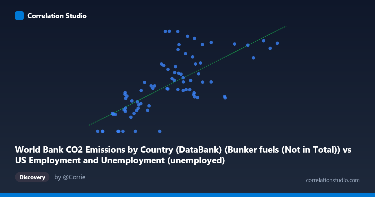
World Bank CO2 Emissions by Country (DataBank) (Bunker fuels (Not in Total)) vs US Employment and Unemployment (unemployed)
- Pearson correlation (r)
- 0.7162
- Spearman correlation
- 0.7324
- p-value
- 0
- Sample size (n)
- 80
- 95% confidence interval
- 0.5892 to 0.8087
- Granger causality
- None
- Granger optimal lag
- 10
AI analysis
Analysis: Bunker Fuel CO₂ Emissions vs. US Unemployment
1. Overall Relationship The scatterplot reveals a moderate-to-strong positive relationship between global bunker fuel CO₂ emissions and US unemployment numbers, with both variables increasing together across the 1941–2020 time span. The linear regression equation (y = 0.101x + 98.45) suggests that for every additional unit of bunker fuel emissions, unemployment rises by roughly 0.10 units. However, the wide scatter around the regression line — particularly in the mid-range of X values (roughly 4,000–9,000) — immediately signals that this is not a tight, mechanistic relationship. Several points deviate substantially from the fitted line, suggesting that a simple linear model captures only part of the story.
2. Correlation Strength, Direction, and Causality The Pearson correlation of r = 0.716 indicates a moderately strong positive association, but the coefficient of determination R² = 0.513 tells a more sobering story: only 51.3% of the variance in US unemployment is statistically explained by bunker fuel emissions. Nearly half the variance remains unexplained by this single predictor. The 95% confidence interval for r [0.589, 0.809] is reasonably tight and excludes zero, and the p-value of 8.1 × 10⁻¹⁴ confirms the correlation is highly statistically significant — this is almost certainly not a chance finding given N = 80 paired observations. Critically, however, the Granger causality tests fail in both directions (X→Y: F = 0.92, p = 0.52; Y→X: F = 0.70, p = 0.72), meaning that neither variable temporally predicts the other with any statistical reliability at the optimal 10-period lag. This is a crucial caveat: statistical significance of correlation does not imply any predictive or causal temporal relationship here.
3. Notable Patterns, Clusters, and Outliers Several structural features stand out in the data. At the lower end of X (roughly 670–2,500), multiple points cluster near Y = 0, representing periods of very low unemployment — likely the wartime and early postwar era (early 1940s–1950s) when both bunker fuel use and unemployment were historically low. A dense mid-range cluster (X ≈ 4,000–9,000) shows considerable vertical spread, with Y values ranging from near 0 to over 1,591 — points like (6,314, 1,591), (5,560, 0), (6,001, 1,590), and (6,982, 1,588) at nearly identical X values but drastically different Y values illustrate that emissions levels alone cannot distinguish high- from low-unemployment periods. At the high end of X (12,000–14,825), values like (14,825, 1,401) and (13,747, 1,441) suggest high bunker emissions paired with elevated but not extreme unemployment, possibly reflecting the 2000s–2010s. The presence of near-zero Y values scattered across the X range is particularly anomalous and warrants scrutiny.
4. Confounding Factors and Interpretive Caveats The most important caveat is that both variables are almost certainly driven by a common underlying factor: time and long-run economic and population growth. Over the 80-year span from 1941 to 2020, global CO₂ emissions from bunker fuels (international shipping and aviation) rose steadily with globalization and trade volume, while US unemployment figures (in absolute numbers, not rates) grew alongside a dramatically expanding labor force. This is a textbook spurious correlation driven by shared secular trends — two independently trending time series will often produce high correlations without any meaningful causal link. Additionally, the axis label assignments appear potentially swapped or metadata-mixed (bunker fuels appearing in a US employment dataset and vice versa), raising data provenance concerns that should be resolved before drawing any conclusions. The zero-valued Y observations (14 points at Y = 0) are also suspicious and may represent missing data coded as zero rather than genuine zero unemployment.
5. Actionable Insights and Further Investigation Given the spurious-correlation risk, the most urgent next step is to detrend both time series (e.g., first-differencing or HP filtering) before recalculating correlation — if r drops substantially after detrending, the relationship is largely an artifact of shared growth trends. Researchers should also verify the dataset column assignments, as the cross-labeling in the metadata (bunker fuels in a US employment file and vice versa) suggests a possible data join error. Replacing absolute unemployment counts with the US unemployment rate would control for labor force growth and provide a more meaningful comparison. Finally, extending the Granger causality test across a range of lags (not just lag 10) and incorporating structural break detection around known shocks — the 1973 oil crisis, 2008–2009 financial crisis, and 2020 COVID pandemic — could reveal whether any localized predictive relationships exist within subperiods, even if none holds globally across the full 80-year window.
X dataset: US Employment and Unemployment
Y dataset: World Bank CO2 Emissions by Country (DataBank)
Part of experiment: Yearly - US Employment and Unemployment vs World Bank CO2 Emissions by Country (DataBank)