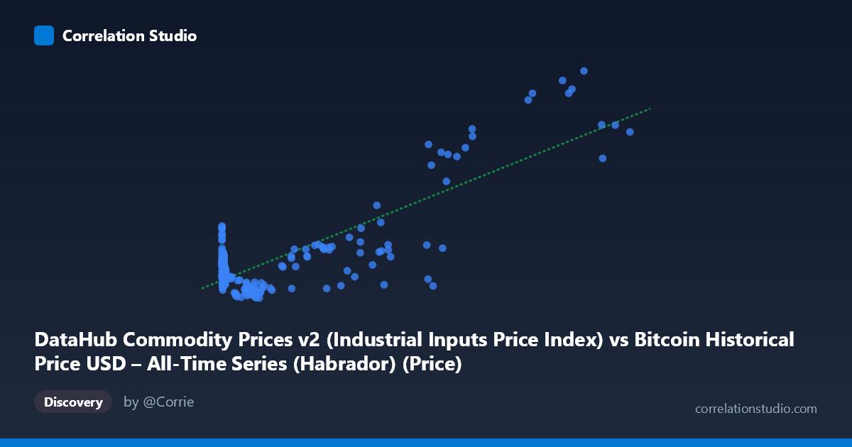
DataHub Commodity Prices v2 (Industrial Inputs Price Index) vs Bitcoin Historical Price USD – All-Time Series (Habrador) (Price)
- Pearson correlation (r)
- 0.8176
- Spearman correlation
- 0.2075
- p-value
- 0
- Sample size (n)
- 182
- 95% confidence interval
- 0.7628 to 0.8607
- Granger causality
- X → Y
- Granger optimal lag
- 4
AI analysis
Analysis: Bitcoin Price vs. Industrial Inputs Price Index
1. Relationship Overview
The scatterplot shows a positive, moderately strong association between Bitcoin's historical USD price (X) and the DataHub Industrial Inputs commodity price index (Y). The relationship is clearly non-linear in raw space — X spans over six orders of magnitude (0.06 to 113,500) while Y ranges narrowly (78.83 to 276.45). Most of the "signal" in the fit comes from the upper tail: as Bitcoin prices climb into the tens of thousands of dollars, the commodity index rises correspondingly into the 110–275 range, while at low Bitcoin prices (under ~$1,000, which dominates the sample by point count), Y stays clustered tightly around 80–115 regardless of X's exact value.
2. Strength, Direction, and Statistical Confidence
The correlation coefficient (r = 0.818, r² = 0.668) indicates a strong positive linear relationship, with the linear model explaining about 67% of the variance in Y — a substantial but incomplete fit, leaving roughly a third of variance unexplained. The 95% CI [0.763, 0.861] is fairly tight and excludes zero, and the p-value of ~0 confirms this correlation is highly unlikely to be due to chance given n=182. However, correlation strength alone doesn't establish causal direction. The Granger causality test suggests X (Bitcoin price) leads Y (commodity index) at a 4-period lag (F=2.71, p=0.032), while the reverse direction is not significant (p=0.281). This is modest evidence of unidirectional predictive value from Bitcoin to commodities, but the F-statistic is not overwhelmingly large, so this should be treated as suggestive rather than definitive.
3. Notable Patterns and Outliers
Several features stand out: (a) a dense cluster of low-X points (X < 1000) where Y hovers between 80–115, showing considerable scatter with no strong local trend — this is likely Bitcoin's early history (2010–2013) overlapping with generally stable commodity prices; (b) a few striking outliers at very low X (0.92, 3.03, 5.00) paired with unusually high Y values (139–142), breaking the general pattern; (c) at high X (90,000), Y values jump to 230–275, but with some inconsistency — e.g., X=58,724 pairs with Y=89.4 (a low outlier) while X=97,365 pairs with Y=260.6, suggesting non-monotonic or lagged behavior at the high end. This scatter at the top suggests the relationship may be driven by a shared time trend rather than a tight functional dependency.
4. Confounding Factors and Caveats
The most important caveat: both series are long-run time series (2010–2025) that have each undergone sustained secular growth (Bitcoin due to adoption/speculation, commodities due to inflation, supply shocks, and post-2020 macro conditions). This is a classic setup for spurious correlation via shared trend/time confounding — both variables trending upward over 15 years will show high r² even without any direct economic linkage. The Granger test's 4-lag result should be interpreted cautiously since financial and commodity series are often non-stationary; without differencing or detrending, Granger causality tests on trending data can produce misleading significance. Additionally, macro factors like USD inflation, global interest rates, and general risk-asset sentiment likely drive both series simultaneously (a common confounder), rather than Bitcoin directly influencing industrial input prices.
5. Suggested Next Steps
To validate whether this is a genuine relationship or trend-driven artifact: (1) re-run correlation and Granger tests on differenced or log-differenced series (returns/growth rates) rather than levels, which removes shared trend bias; (2) include a control for a common macro variable (e.g., USD index, CPI, or global M2 money supply) to test if the X-Y link survives after partialling out inflation; (3) segment the analysis by era (pre-2017, 2017–2020, 2020+) to check whether the relationship is stable or driven by a specific regime (e.g., the 2020–2021 bull run); and (4) apply a log transform to X given its multi-order-of-magnitude range, which may reveal a cleaner, more interpretable functional form than the current linear fit.
X dataset: Bitcoin Historical Price USD – All-Time Series (Habrador)
Y dataset: DataHub Commodity Prices v2
Part of experiment: Bitcoin - Bitcoin Historical Price USD – All-Time Series (Habrador) vs DataHub Commodity Prices v2