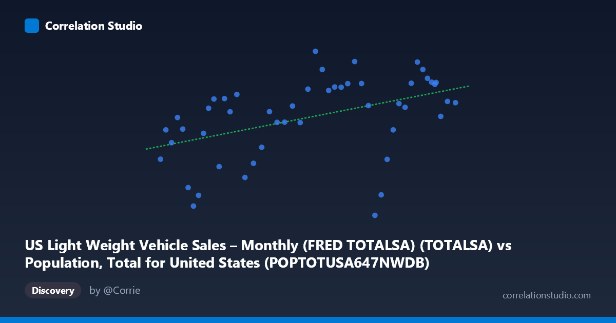
US Light Weight Vehicle Sales – Monthly (FRED TOTALSA) (TOTALSA) vs Population, Total for United States (POPTOTUSA647NWDB) (POPTOTUSA647NWDB)
- Pearson correlation (r)
- 0.4484
- Spearman correlation
- 0.5258
- p-value
- 0.001233
- Sample size (n)
- 49
- 95% confidence interval
- 0.1913 to 0.6479
- Granger causality
- None
- Granger optimal lag
- 1
- Time coverage
- 1976-01-01 to 2024-01-01
- Recomputed on refreshed data
- 2026-10-07 (r was 0.4352)
AI analysis
Analysis: US Population vs. Light Vehicle Sales
Relationship Overview The scatterplot reveals a modest positive relationship between US total population (X-axis) and monthly light-weight vehicle sales in SAAR terms (Y-axis). As population grows over the 1976–2024 study window, vehicle sales show a general upward tendency, which is intuitively plausible — a larger population creates a larger pool of potential vehicle buyers. However, the scatter is considerable, and the relationship is far from deterministic. The linear regression equation (y = 2.46×10⁻⁸x + 8.18) implies that each additional million people in the US population is associated with roughly a 0.025 million unit increase in annualized vehicle sales, a modest marginal effect.
Correlation Strength and Statistical Framing The Pearson correlation of r = 0.435 indicates a weak-to-moderate positive association. More critically, r² = 0.189 means that population size explains only about 19% of the variance in vehicle sales — leaving roughly 81% of the variation driven by other factors. The 95% confidence interval for r spans [0.175, 0.638], a fairly wide range that reflects meaningful uncertainty about the true population-level relationship, though it is entirely positive, ruling out a negative association with reasonable confidence. The p-value of 0.00178 confirms statistical significance at conventional thresholds (p < 0.05), so the positive association is unlikely to be a pure artifact of sampling chance given n = 49 paired observations. That said, statistical significance should not be conflated with practical importance — 19% explained variance leaves the bulk of sales dynamics unexplained by demographics alone. Granger causality tests show no significant predictive directionality in either direction (X→Y: F = 0.633, p = 0.430; Y→X: F = 0.580, p = 0.450), meaning that population does not reliably lead vehicle sales temporally, nor does sales activity predict population growth. This effectively rules out a straightforward temporal causal mechanism between the two series at a 1-period lag.
Notable Patterns, Clusters, and Outliers Several features stand out visually. There is a lower-left cluster of points (population ~218M–245M, sales ~10–13M units) corresponding broadly to the late 1970s and early 1980s, a period marked by oil shocks and recession-driven sales suppression. A central-to-upper-right cluster (population ~270M–310M, sales ~15–18M) reflects the mid-1990s through mid-2000s boom years. Two points are particularly notable outliers: (306,771,529; 9.79) — very low sales despite a relatively large population, likely corresponding to the 2008–2009 financial crisis collapse in auto demand — and (282,162,411; 18.64), representing peak sales performance around the 2015–2016 era of historically low interest rates and post-recession pent-up demand. The point (231,664,000; 10.29) in the lower-left also likely reflects early-1980s recession conditions. These outliers powerfully illustrate that macroeconomic shocks can overwhelm demographic trends entirely.
Confounding Factors and Caveats Several important caveats apply. First, both variables are strongly trended over time — population grows monotonically while vehicle sales follow broader economic cycles — creating a classic spurious correlation risk driven by shared time trends rather than a direct causal mechanism. Second, vehicle sales are heavily influenced by interest rates, fuel prices, consumer confidence, credit availability, and fleet replacement cycles, none of which are captured here. Third, population composition matters as much as total population: an aging demographic or rising urbanization (with reduced car dependency) can depress per-capita demand even as total population grows. Fourth, SAAR methodology in the vehicle sales series introduces its own adjustments that may not align cleanly with annual population snapshots. Finally, the wide confidence interval for r suggests that with different sampling years, the observed correlation could vary substantially.
Actionable Insights and Further Investigation Given that population alone explains less than one-fifth of vehicle sales variance and shows no Granger-causal relationship, researchers and analysts should prioritize macroeconomic controls — particularly interest rates, real disposable income, and consumer sentiment indices — when modeling vehicle demand. A multiple regression or time-series model (e.g., VAR or ARIMAX) incorporating GDP growth, credit conditions, and fuel costs would almost certainly yield far stronger predictive power. It would also be valuable to detrend both series before computing correlation to isolate cyclical co-movement from shared time trends, and to examine per-capita vehicle sales rather than absolute totals to control for population growth mechanically. Segmenting the analysis by decade or economic regime (pre/post-2008, pre/post-COVID) could reveal whether the population–sales relationship has structurally changed over time, particularly as remote work, ride-sharing, and EV adoption reshape vehicle ownership patterns.
X dataset: Population, Total for United States (POPTOTUSA647NWDB)
Y dataset: US Light Weight Vehicle Sales – Monthly (FRED TOTALSA)
Part of experiment: Yearly - Population, Total for United States (POPTOTUSA647NWDB) vs US Light Weight Vehicle Sales – Monthly (FRED TOTALSA)