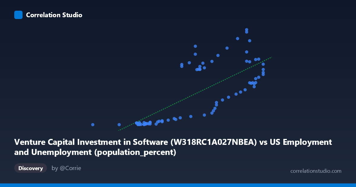
Venture Capital Investment in Software (W318RC1A027NBEA) vs US Employment and Unemployment (population_percent)
- Pearson correlation (r)
- 0.7474
- Spearman correlation
- 0.7645
- p-value
- 0
- Sample size (n)
- 79
- 95% confidence interval
- 0.6305 to 0.8312
- Granger causality
- None
- Granger optimal lag
- 10
- Time coverage
- 1946-01-01 to 2024-01-01
AI analysis
Scatterplot Analysis: Venture Capital Investment in Software vs. US Employment (Population Percent)
Relationship Overview
The scatterplot reveals a moderately strong positive relationship between Venture Capital (VC) investment in software and US employment as a percentage of population, spanning nearly eight decades (1946–2024). As VC investment in software increases, employment population percentage tends to rise correspondingly. However, the relationship is notably heteroscedastic — the spread of Y values widens considerably at higher X values (above ~62–63 on the X-axis), suggesting that the relationship becomes less predictable as investment scales up. The linear regression equation (y = 35.49x − 2069.21) implies that each unit increase in software VC investment is associated with roughly 35.5 percentage points of employment population share, though this mechanistic interpretation requires caution given the observational nature of the data.
Correlation Strength and Statistical Significance
The Pearson correlation of r = 0.747 indicates a moderately strong positive association, and the p-value of 2.44×10⁻¹⁵ confirms this is extraordinarily unlikely to be a chance finding at any conventional significance threshold. The 95% confidence interval [0.63, 0.83] is reasonably tight, suggesting reliable estimation even across this 79-year span. That said, R² = 0.559 means that roughly 56% of the variance in employment population percentage is explained by software VC investment — leaving 44% attributable to other factors. This is a meaningful but incomplete explanatory relationship. Critically, the Granger causality analysis finds no significant directional predictive relationship in either direction (X→Y: F = 2.01, p = 0.053; Y→X: F = 1.08, p = 0.40). The X→Y direction narrowly misses conventional significance (p just above 0.05 at optimal lag = 10 periods), meaning we cannot confidently assert that software investment temporally precedes and predicts employment changes — co-movement driven by a shared underlying trend is a more defensible interpretation.
Notable Patterns, Clusters, and Outliers
The data separates visually into two distinct clusters: a low-X, low-Y cluster (X ≈ 55.8–61.5, Y ≈ 0.85–35) corresponding to earlier decades with minimal software investment, and a high-X, high-Y cluster (X ≈ 62–67, Y ≈ 40–466) reflecting the post-1980s technology era. Within the upper cluster, variance in Y is enormous — for instance, at X ≈ 62.6–62.9, Y values range from ~40 to ~385, and at X ≈ 66.0, Y spans from ~311 to ~466. This fan-shaped dispersion signals heteroscedasticity and potential non-linearity, suggesting a log or power transformation of Y might improve model fit. Several points stand out as outliers: (66.0, 466.42) and (65.4, 422.88) sit well above the regression line, while (62.3, 40.98) and (63.7, 57.64) fall unexpectedly low for their X values, indicating periods where high investment did not translate to proportional employment gains.
Confounding Factors and Interpretive Caveats
The most significant caveat here is the shared secular trend problem: both VC investment in software and employment population rates grew substantially over the post-war period, largely driven by the same macroeconomic forces — GDP growth, demographic shifts, technological diffusion, and policy changes. This means the correlation may substantially reflect spurious co-trending rather than a direct causal mechanism. The dataset labels also appear potentially swapped or cross-referenced in an unusual way (X is labeled as VC investment but sourced from an employment dataset, and vice versa), which warrants verification before drawing firm conclusions. Additionally, employment population percentage is influenced by labor force participation rates, demographics (Baby Boom cohort aging), gender workforce integration, and recessionary cycles — factors entirely independent of software investment. The 10-period Granger lag is also quite long (10 years), which may reflect indirect structural relationships rather than direct causal pathways.
Actionable Insights and Further Investigation
Given the absence of confirmed Granger causality, analysts should avoid using this correlation to justify direct investment-to-employment policy claims without controlling for confounders. Priority next steps should include: (1) detrending both series (e.g., first-differencing or HP filtering) to test whether correlation persists after removing shared secular trends; (2) applying a log transformation to Y to address the apparent exponential growth pattern and heteroscedasticity; (3) incorporating control variables such as GDP growth, inflation, and labor force participation to isolate the software investment channel; and (4) segmenting the analysis by era (pre-/post-1980, pre-/post-dot-com, pre-/post-2008) to test whether the relationship is stable across different technological and economic regimes. A vector autoregression (VAR) or cointegration framework would be a more rigorous approach than Granger causality alone for assessing long-run dynamic relationships between these two time series.
X dataset: US Employment and Unemployment
Y dataset: Venture Capital Investment in Software
Part of experiment: Yearly - US Employment and Unemployment vs Venture Capital Investment in Software