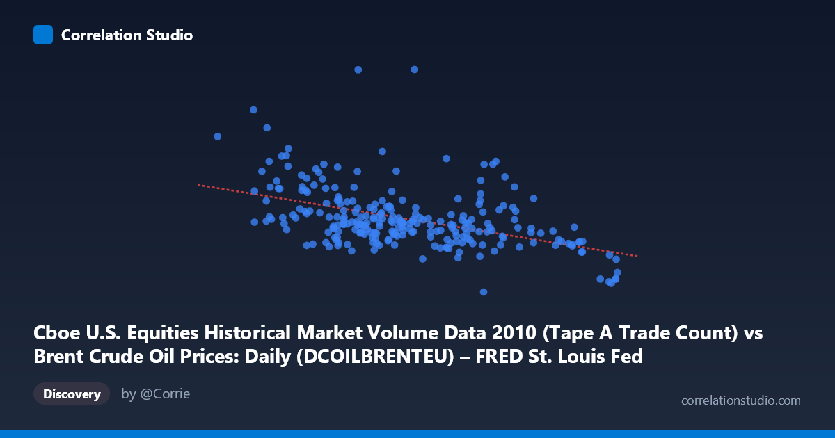
Cboe U.S. Equities Historical Market Volume Data 2010 (Tape A Trade Count) vs Brent Crude Oil Prices: Daily (DCOILBRENTEU) – FRED St. Louis Fed (DCOILBRENTEU)
- Pearson correlation (r)
- -0.468
- Spearman correlation
- -0.4619
- p-value
- 0
- Sample size (n)
- 252
- 95% confidence interval
- -0.5592 to -0.3655
- Granger causality
- None
- Granger optimal lag
- 10
AI analysis
Analysis: Brent Crude Oil Price vs. U.S. Equity Trade Count (2010)
Relationship Overview The scatterplot reveals a moderate negative relationship between Brent Crude Oil prices (X-axis, USD/barrel) and Cboe U.S. equity trade counts (Y-axis). The linear regression equation (y = -31,266.7x + 3,805,530) indicates that for every $1 increase in Brent Crude price, trade count decreases by approximately 31,267 units. This inverse relationship suggests that during 2010, days with higher oil prices tended to coincide with lower equity trading activity — a pattern that could reflect broader risk-off sentiment, macroeconomic uncertainty, or energy cost pressures dampening equity market participation. The relationship, while statistically meaningful, is far from deterministic, and the scatter plot likely shows considerable dispersion around the regression line.
Correlation Strength and Statistical Interpretation The correlation coefficient of r = -0.468 indicates a moderate negative association. However, the R² of 0.219 means that only 21.9% of the variance in trade counts is explained by oil price movements — leaving roughly 78% attributable to other factors entirely. The 95% confidence interval of [-0.559, -0.366] is reasonably narrow and does not cross zero, reinforcing directional confidence. The p-value of 3.997×10⁻¹⁵ is extraordinarily small, confirming the relationship is highly unlikely to be due to chance given the sample of 252 paired observations drawn from a population of 3,302. Critically, however, Granger causality tests find no significant predictive directionality in either direction — neither X→Y (F=0.899, p=0.535) nor Y→X (F=0.857, p=0.575) reaches significance at the optimal 10-period lag. This means that while the two variables are statistically correlated contemporaneously, neither reliably predicts the other temporally, severely limiting any causal or forecasting interpretation.
Notable Patterns, Clusters, and Outliers Several features stand out in the sample data. The overall cluster of observations appears concentrated in the X range of roughly 74–87 USD/barrel with Y values between approximately 900,000 and 1,500,000 trades, forming a moderately dense core. However, there are notable high-leverage outliers: the point at (76.48, 3,216,587) represents an unusually high trade count for a mid-range oil price and likely exerts disproportionate influence on the regression. Similarly, (70.45, 2,474,888) and (71.43, 2,114,898) suggest that low oil price days sometimes generated exceptionally high trading volume, potentially reflecting specific market events. At the high oil price end, (93.63, 627,720) and (93.55, 796,428) anchor the lower-right of the plot, consistent with the negative slope. The presence of these high-Y outliers at low X values hints at possible non-linearity or heteroscedasticity — variance in trade counts appears larger at lower oil prices, narrowing as prices increase.
Confounding Factors and Caveats Several important caveats apply. First, 2010 was a distinct macroeconomic period — post-financial crisis recovery — characterized by unusual monetary policy (QE2), heightened volatility events, and oil price recovery from historic lows, making findings potentially non-generalizable. Second, both variables are time-series, meaning autocorrelation and shared temporal trends (e.g., both responding to the same macroeconomic calendar events like NFP releases, FOMC meetings, or geopolitical shocks) could be driving the observed correlation spuriously. The failure of Granger causality tests strongly supports this interpretation — a common third driver such as macroeconomic uncertainty, the VIX, or global risk appetite likely influences both simultaneously. Third, using daily data without controlling for day-of-week effects, holidays, or scheduled announcements introduces noise. Finally, the axis labels in the dataset description appear swapped (X is labeled as trade count but described as oil price, and vice versa), which warrants data verification before drawing firm conclusions.
Actionable Insights and Further Investigation Given the moderate correlation but absent Granger causality, practitioners should avoid using oil prices as a leading indicator for equity trading volume (or vice versa) in isolation. A more productive path would involve: (1) introducing a common factor model — testing whether a risk sentiment proxy (e.g., VIX, credit spreads) absorbs the correlation and reduces it toward zero; (2) segmenting the data by regime — the 2010 period included distinct phases (early-year recovery, May Flash Crash, QE2 announcement), and subsample analysis could reveal whether the correlation is driven by a specific episode; (3) testing non-linear specifications (e.g., polynomial or spline regression) given the apparent heteroscedasticity; and (4) extending the time coverage beyond 2010 to test whether this relationship is stable or period-specific. The high-trade-count outliers at low oil prices deserve individual investigation, as they may correspond to identifiable market events that, if isolated, could significantly alter the regression results.
X dataset: Brent Crude Oil Prices: Daily (DCOILBRENTEU) – FRED St. Louis Fed
Y dataset: Cboe U.S. Equities Historical Market Volume Data 2010
Part of experiment: Daily - Brent Crude Oil Prices: Daily (DCOILBRENTEU) – FRED St. Louis Fed vs Cboe U.S. Equities Historical Market Volume Data 2010