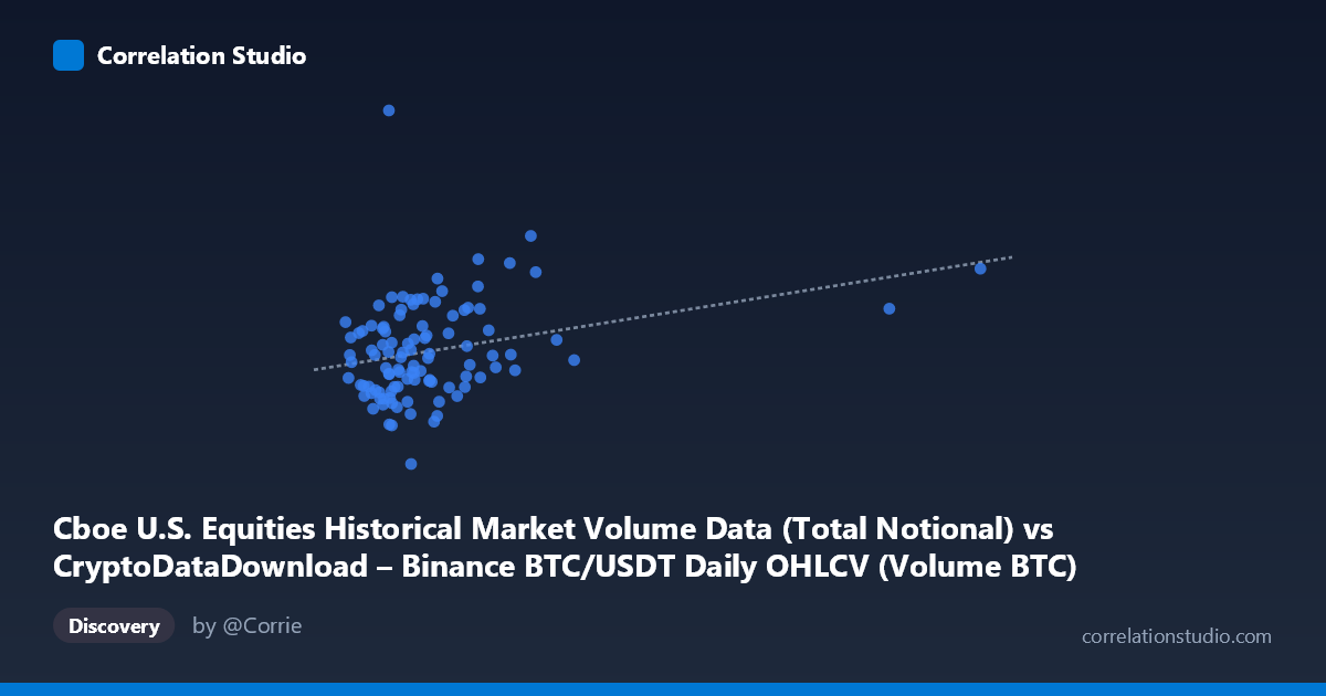
Cboe U.S. Equities Historical Market Volume Data (Total Notional) vs CryptoDataDownload – Binance BTC/USDT Daily OHLCV (Volume BTC)
- Pearson correlation (r)
- 0.2847
- Spearman correlation
- 0.2696
- p-value
- 0.003402
- Sample size (n)
- 104
- 95% confidence interval
- 0.0974 to 0.4525
- Granger causality
- None
- Granger optimal lag
- 10
AI analysis
Analysis: Cboe Equities Volume vs. Binance BTC/USDT Volume
1. Overview of the Relationship
The scatterplot shows a modest positive association between the two variables: as the X variable (labeled here as Cboe notional volume, though the underlying data appears to be Binance-derived) increases, Y tends to increase as well, but the relationship is loose and noisy rather than tight. Most of the data points cluster in the lower-X range (10,000–30,000), with a long right tail extending to a few high-X outliers (near 92,500 and 106,300). The bulk of the cloud shows substantial vertical scatter at any given X value, indicating that X alone is a weak predictor of Y across most of the observed range.
2. Strength, Direction, and Statistical Confidence
The correlation coefficient (r = 0.408) indicates a weak-to-moderate positive linear relationship. The r² of 0.167 means only about 16.7% of the variance in Y is explained by X — the remaining ~83% is driven by other factors, noise, or nonlinear dynamics not captured by this simple linear model. The 95% confidence interval [0.220, 0.567] is fairly wide but excludes zero, and the p-value (6.5×10⁻⁵) is well below conventional significance thresholds, so the correlation is statistically real rather than a chance artifact of this 90-point sample. However, statistical significance should not be conflated with practical strength: this is a real but weak relationship, not one suitable for precise prediction. Critically, the Granger causality tests (optimal lag = 10 periods) show no significant predictive direction in either direction (X→Y: p=0.41; Y→X: p=0.68). This means that despite the contemporaneous correlation, neither series reliably helps forecast future values of the other — the relationship is likely coincidental co-movement, shared exposure to a common external driver, or a static/structural association rather than a lead-lag dynamic.
3. Notable Patterns and Outliers
Several features stand out: (1) A visible low-Y outlier near X≈20,300 with Y≈34.0 billion, far below the general trend line — this point pulls down the fit locally. (2) High-X outliers at X≈92,500 and X≈106,300 have relatively high Y values (~61B and ~68B respectively), lending support to the positive slope but with very few points anchoring that region — meaning the regression line's behavior at high X is driven by a handful of observations and is less reliable there. (3) The dense low-X cluster (10,000–30,000) itself shows Y ranging widely from ~34B to ~70B, suggesting high intrinsic variability in Y that's largely independent of X in this region. There's no obvious nonlinear curvature (e.g., saturation or threshold effects) beyond what a straight line captures, though the sparse high-X tail makes it hard to rule out nonlinearity definitively.
4. Confounding Factors and Caveats
Several caveats limit interpretation: the metadata labeling is internally inconsistent — X is described as "Cboe Equities... Total Notional" while its dataset name references Binance BTC/USDT OHLCV, and Y is labeled "Volume BTC" but tied to the Cboe dataset. This suggests a possible mismatch or mislabeling in the data pipeline that should be verified before drawing substantive conclusions about what's actually being compared (equities volume vs. crypto volume, or two crypto-derived series). Additionally, both series may be affected by common macro drivers (e.g., overall market volatility, risk-on/risk-off sentiment, weekday/weekend effects, or shared calendar effects like month-end volume spikes) that could produce spurious correlation without direct causal linkage. The small sample (n=90) relative to the full population (N=1,980) and the short time coverage (Jan–May 2026) also limit generalizability — seasonal or regime-specific effects during this window may not hold across the full dataset.
5. Actionable Recommendations
Before relying on this relationship: (1) verify and correct the axis/dataset labeling to ensure the correct series are being compared. (2) Given the null Granger causality result, avoid using one series to forecast the other; instead, investigate whether both are driven by a shared latent factor (e.g., overall trading activity, volatility index, or macro liquidity conditions) via a multivariate model. (3) Examine the low-Y and high-X outliers individually — check for data entry errors, holidays, or exchange-specific anomalies on those particular dates. (4) Expand the time window and sample size (using more of the full N=1,980 population) to test whether r² and the confidence interval stabilize or shift, which would clarify if the current weak correlation is a robust structural feature or a short-window artifact. (5) Consider nonlinear or lagged-feature models (beyond the tested lags) and control variables (volatility, day-of-week) to see if explained variance improves meaningfully beyond 16.7%.
X dataset: CryptoDataDownload – Binance BTC/USDT Daily OHLCV
Y dataset: Cboe U.S. Equities Historical Market Volume Data
Part of experiment: Bitcoin - CryptoDataDownload – Binance BTC/USDT Daily OHLCV vs Cboe U.S. Equities Historical Market Volume Data