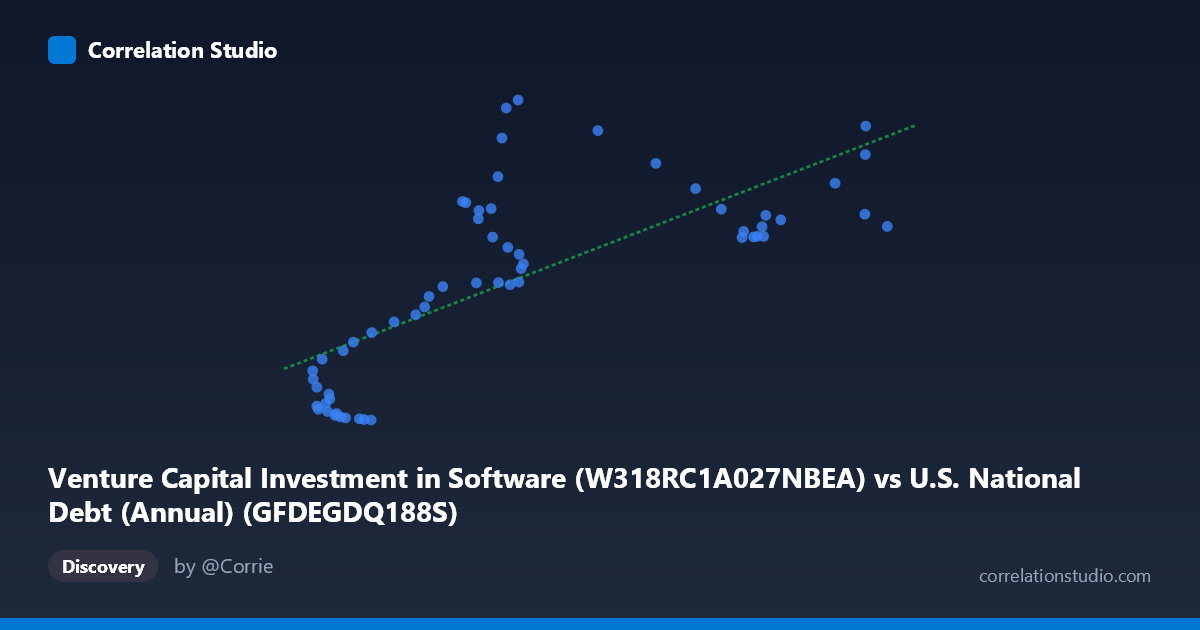
Venture Capital Investment in Software (W318RC1A027NBEA) vs U.S. National Debt (Annual) (GFDEGDQ188S)
- Pearson correlation (r)
- 0.7157
- Spearman correlation
- 0.7639
- p-value
- 0
- Sample size (n)
- 59
- 95% confidence interval
- 0.5627 to 0.8212
- Granger causality
- None
- Granger optimal lag
- 10
AI analysis
Analysis: Venture Capital Software Investment vs. U.S. National Debt (% GDP)
Relationship Overview
The scatterplot reveals a moderately positive relationship between Venture Capital (VC) investment in software and the U.S. National Debt as a percentage of GDP over the period 1966–2024. As VC software investment increases, federal debt as a share of GDP tends to rise as well. The linear regression equation (y = 3.345x − 2.98) suggests that for each unit increase in VC software investment, national debt as a percent of GDP increases by approximately 3.35 percentage points on average. However, the scatter around this trend line is substantial, and the data cloud shows meaningful dispersion, particularly in the mid-range of X values, hinting that this relationship is far from deterministic.
Correlation Strength and Statistical Interpretation
The Pearson correlation of r = 0.716 indicates a moderately strong positive association, though the explanatory power tells a more cautious story: r² = 0.512, meaning that VC software investment accounts for only about 51.2% of the variance in national debt-to-GDP ratio. Nearly half the variation remains unexplained by this single predictor. The 95% confidence interval for r spans [0.563, 0.821], which is notably wide, reflecting meaningful uncertainty in the true population correlation — the relationship could be considerably weaker or stronger than the point estimate suggests. The p-value of 1.89 × 10⁻¹⁰ is highly significant, confirming this correlation is extremely unlikely to be a chance artifact in a sample of this size (n = 59). Critically, however, the Granger causality tests fail in both directions — neither X→Y (F = 1.79, p = 0.109) nor Y→X (F = 1.14, p = 0.367) reaches significance at the optimal 10-period lag. This means the correlation, while statistically robust in a cross-sectional sense, carries no demonstrable temporal predictive power: knowing past VC investment does not reliably forecast future debt levels, and vice versa.
Patterns, Clusters, and Outliers
The data visually cluster into two somewhat distinct regions. A low-X, low-to-moderate-Y cluster appears in the range X ≈ 30–50, where Y values span widely from roughly 11 to 135, suggesting high variability in national debt levels when VC investment was historically low. A higher-X, moderate-to-high-Y cluster emerges around X ≈ 55–125, where Y generally ranges from 200 to 466, indicating the post-1990s era when both software investment and national debt expanded together. Several notable outliers are visible: points near (62, 455), (64, 466), and (77, 423) show extremely high Y values relative to their X position, while points like (35, 15), (34, 20), and (38, 13) represent unusually low debt levels for their VC investment levels. The non-linear character of the spread — with greater Y variance at middle X values — suggests potential heteroscedasticity, which could undermine the linear model's reliability across the full range.
Confounding Factors and Caveats
This correlation almost certainly reflects shared temporal trends rather than a genuine causal mechanism. Both variables have grown substantially since the 1980s–1990s, driven by macroeconomic forces entirely independent of one another: national debt has been shaped by defense spending, entitlement programs, recessions, and tax policy, while VC software investment has been driven by the digital revolution, interest rate environments, and technological adoption cycles. This is a textbook case of spurious correlation via common time trend — two series that both generally increase over decades will inevitably correlate. The failed Granger tests reinforce this interpretation. Additionally, the dataset mismatch in labeling (axis labels appear swapped in the metadata) warrants scrutiny before drawing any conclusions. The wide confidence interval and high residual variance further caution against over-interpreting the regression slope.
Actionable Insights and Further Investigation
Given the likely spurious nature of this correlation, the most productive next steps would involve detrending both series (e.g., using first differences or percent changes year-over-year) before re-examining correlation, which would strip out the shared upward drift. Researchers should introduce control variables — GDP growth rate, federal funds rate, and major fiscal events (wars, financial crises) — to test whether any partial correlation survives. Extending the Granger causality analysis with different lag structures or using a Vector Autoregression (VAR) framework could provide more nuanced temporal insights. Finally, regime segmentation (pre/post-2000, or pre/post-2008 financial crisis) may reveal whether the relationship strengthens or disappears within specific economic eras, which would be more actionable for policy or investment analysis than the pooled 58-year trend.
X dataset: U.S. National Debt (Annual)
Y dataset: Venture Capital Investment in Software
Part of experiment: Yearly - U.S. National Debt (Annual) vs Venture Capital Investment in Software