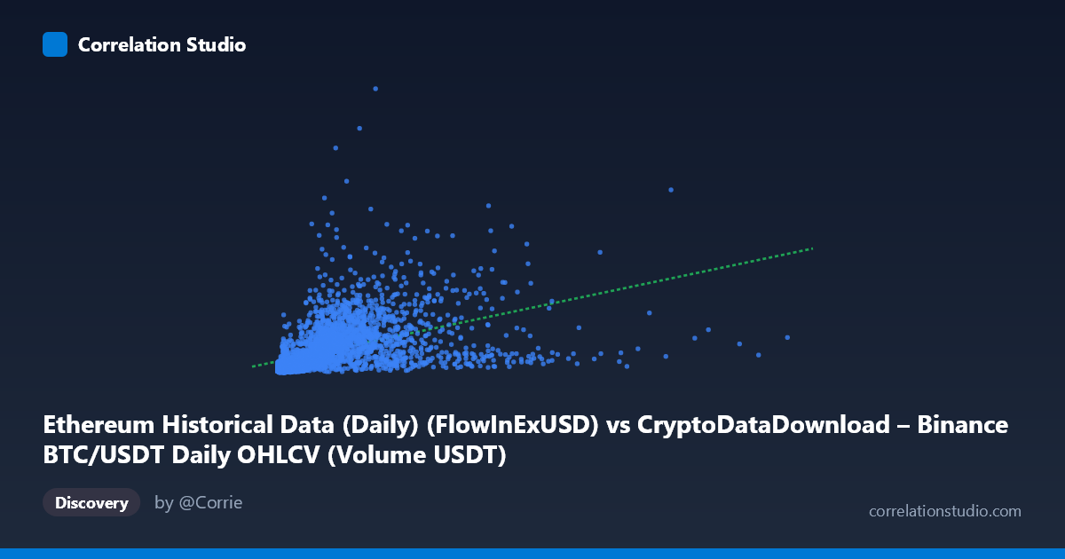
Ethereum Historical Data (Daily) (FlowInExUSD) vs CryptoDataDownload – Binance BTC/USDT Daily OHLCV (Volume USDT)
- Pearson correlation (r)
- 0.4644
- Spearman correlation
- 0.7333
- p-value
- 0
- Sample size (n)
- 3191
- 95% confidence interval
- 0.4367 to 0.4912
- Granger causality
- None
- Granger optimal lag
- 10
- Time coverage
- 2017-08-17 to 2026-05-20
AI analysis
Analysis: Ethereum Flow-In vs. Binance BTC/USDT Volume
1. Relationship Overview
The scatterplot depicts a moderate positive association between Ethereum's daily flow-in (USD) and Binance BTC/USDT trading volume (USDT). Both variables span multiple orders of magnitude (X: ~$1M to $17.5B; Y: ~$14M to $6.9B), with heavily right-skewed distributions — the vast majority of points cluster in the lower-left region (under ~$5B on X, under ~$1B on Y), while a sparse tail of extreme values stretches toward the upper right. This pattern, combined with the note that Spearman's ρ exceeds Pearson's r, strongly suggests the true relationship is monotonic but non-linear (likely logarithmic or power-law), consistent with how crypto market activity metrics typically scale.
2. Strength, Direction, and Uncertainty
The Pearson correlation (r = 0.4644) indicates a moderate positive linear relationship, but r² = 0.2157 reveals that only about 21.6% of the variance in BTC volume is explained by ETH flow-in — leaving nearly 80% attributable to other factors or non-linear structure not captured by this simple metric. The 95% CI [0.437, 0.491] is tight and the p-value is effectively 0, confirming the correlation is statistically robust and not a product of chance, even though its practical explanatory power is limited. Critically, the Granger causality tests (F = 0.86, p = 0.57 for X→Y; F = 1.03, p = 0.41 for Y→X) show no significant predictive direction in either direction at the tested 10-lag horizon. This means that despite the contemporaneous correlation, past values of one series do not meaningfully help forecast future values of the other — the co-movement is likely driven by shared external market dynamics rather than one variable causing the other over time.
3. Patterns, Clusters, and Outliers
The sample points reveal a dense cluster of low-to-moderate values (X < $1B, Y < $500M) representing typical daily activity, with a linear regression slope of 0.15 fitting the bulk reasonably. However, several notable outliers exist: points like (5.07B, 232M) and (1.92B, 157M) show high X with disproportionately low Y, while (7.16B, 1.79B) and (3.4B, 1.57B) sit further along both axes, suggesting occasional co-spikes during high-volatility trading periods. The heteroscedastic fan-shaped spread — variance in Y increasing with X — is typical of financial volume data and reinforces the case for a log-log transformation before further linear modeling.
4. Confounding Factors and Caveats
Both variables are volume/flow metrics denominated in USD/USDT from the crypto market, meaning they are likely both driven by common macro factors: overall market sentiment, BTC/ETH price rallies, exchange liquidity events, regulatory news, and stablecoin flows. This shared dependency on broader "crypto market activity" is a classic confounder that can inflate correlation without implying direct causal linkage. Additionally, using raw (non-log) values in a Pearson correlation is problematic given the multiple-order-of-magnitude range and skew — this can distort both the r estimate and the linear regression fit, as hinted by the Spearman/Pearson discrepancy. The time span (2017–2026) also covers vastly different market regimes (bull/bear cycles, differing volume baselines), so pooling all data may mask regime-dependent relationships.
5. Recommendations for Further Investigation
1. Re-run correlation and regression on log-transformed variables (log(X), log(Y)) to better capture the apparent power-law relationship and obtain a more accurate r²/fit. 2. Segment by market regime or time period (e.g., yearly or bull/bear phases) to check whether the correlation strength is stable or regime-dependent. 3. Investigate common confounders directly — such as BTC/ETH price level, total crypto market cap, or stablecoin supply — to test whether they better explain the shared variance than a direct X-Y relationship. 4. Extend Granger causality testing to shorter lags (1–3 days) and consider non-linear causality tests (e.g., transfer entropy), since the linear Granger framework may miss non-linear predictive signals. 5. Flag and investigate outlier days (e.g., the high-X/low-Y points) for specific market events (exchange outages, flash crashes, airdrops) that may explain the divergence from the general trend.
X dataset: CryptoDataDownload – Binance BTC/USDT Daily OHLCV
Y dataset: Ethereum Historical Data (Daily)
Part of experiment: Bitcoin - CryptoDataDownload – Binance BTC/USDT Daily OHLCV vs Ethereum Historical Data (Daily)