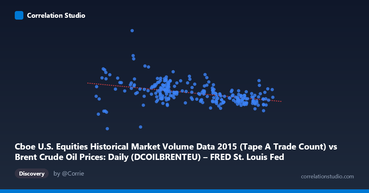
Cboe U.S. Equities Historical Market Volume Data 2015 (Tape A Trade Count) vs Brent Crude Oil Prices: Daily (DCOILBRENTEU) – FRED St. Louis Fed (DCOILBRENTEU)
- Pearson correlation (r)
- -0.4039
- Spearman correlation
- -0.4814
- p-value
- 0
- Sample size (n)
- 251
- 95% confidence interval
- -0.5026 to -0.2948
- Granger causality
- None
- Granger optimal lag
- 10
AI analysis
Analysis: Cboe U.S. Equities Trade Count vs. Brent Crude Oil Price (2015)
Relationship Overview The scatterplot reveals a moderate negative relationship between the Cboe U.S. Equities Tape A Trade Count (X) and Brent Crude Oil prices (Y) across 2015. The linear regression equation (y = −12,919.1x + 2,104,170) indicates that higher daily trade counts on U.S. equity exchanges tend to coincide with lower Brent crude prices, and vice versa. Visually, the data shows a downward-sloping trend, but with considerable scatter — the relationship is real but far from deterministic. The spread of points across the full range of X values makes it immediately clear that trade count alone is a poor direct predictor of oil price.
Correlation Strength and Statistical Significance The Pearson correlation of r = −0.404 confirms a moderate negative association, but the R² of 0.163 means only 16.3% of the variance in Brent crude prices is explained by equity trade volume — leaving roughly 83.7% unexplained by this variable alone. The 95% confidence interval of [−0.503, −0.295] is relatively tight and does not cross zero, and the p-value of 2.889×10⁻¹¹ confirms the correlation is highly statistically significant, ruling out random chance given n = 251 paired observations. However, statistical significance here is partly a function of the large population (N = 3,302) and adequate sample size — significance does not imply practical or causal importance. Critically, Granger causality tests find no significant predictive direction in either direction (X→Y: F = 0.565, p = 0.841; Y→X: F = 0.323, p = 0.975), meaning neither variable temporally predicts the other at any tested lag up to 10 periods. This strongly cautions against any causal interpretation.
Notable Patterns, Clusters, and Outliers Several features stand out in the data. There is a visible clustering of points in the 45–55 trade count range with a wide vertical spread in oil prices (roughly 1.1M–2.1M barrels-equivalent price range), suggesting high variability in oil prices even when equity trading activity is moderate. At the high end of X (60–66), oil prices tend to cluster in a lower band (~1.0M–1.5M), consistent with the negative slope. A few notable outliers are apparent: the point near (43.84, 2,076,907) and (41.86, 2,247,816) represent days with low trade counts but unusually high oil price readings, pulling the regression line and potentially inflating the correlation magnitude. The point at (37.22, 576,208) is an extreme low on both axes and may represent a holiday-shortened or anomalous trading session that warrants separate examination.
Confounding Factors and Caveats This correlation is highly susceptible to confounding by shared time-series trends. In 2015, Brent crude oil experienced a well-documented secular price decline from ~$60 to below $40 per barrel, while equity market volatility (and therefore trading volumes) fluctuated in response to macroeconomic events, Federal Reserve policy signals, and global risk sentiment. Both variables are likely responding to common underlying drivers — such as economic uncertainty, risk-off behavior, or commodity market stress — rather than influencing each other directly. Seasonality, day-of-week effects, and market microstructure factors (e.g., algorithmic trading surges on volatile days) could all independently affect trade counts. The axes also appear somewhat mismatched in labeling (the dataset descriptions suggest the X and Y assignments may reflect a quirk in data joining), which adds interpretive caution.
Actionable Insights and Further Investigation Given the absence of Granger causality, practitioners should not use equity trade count as a leading indicator of oil prices (or vice versa) for short-term trading strategies. Further investigation should include: (1) controlling for calendar effects and known macro events (e.g., OPEC announcements, Fed meetings) to isolate residual correlation; (2) testing non-linear models (e.g., polynomial or spline regression) given the visible heteroscedasticity and potential clustering; (3) examining whether the relationship strengthens during high-volatility regimes versus calm periods using a rolling-window correlation; and (4) incorporating additional variables such as the VIX, USD index, or energy sector ETF flows to build a more explanatory multivariate model. The 16.3% R² suggests meaningful signal exists, but it is likely a proxy for shared macroeconomic stress rather than a direct financial linkage.
X dataset: Brent Crude Oil Prices: Daily (DCOILBRENTEU) – FRED St. Louis Fed
Y dataset: Cboe U.S. Equities Historical Market Volume Data 2015
Part of experiment: Daily - Brent Crude Oil Prices: Daily (DCOILBRENTEU) – FRED St. Louis Fed vs Cboe U.S. Equities Historical Market Volume Data 2015