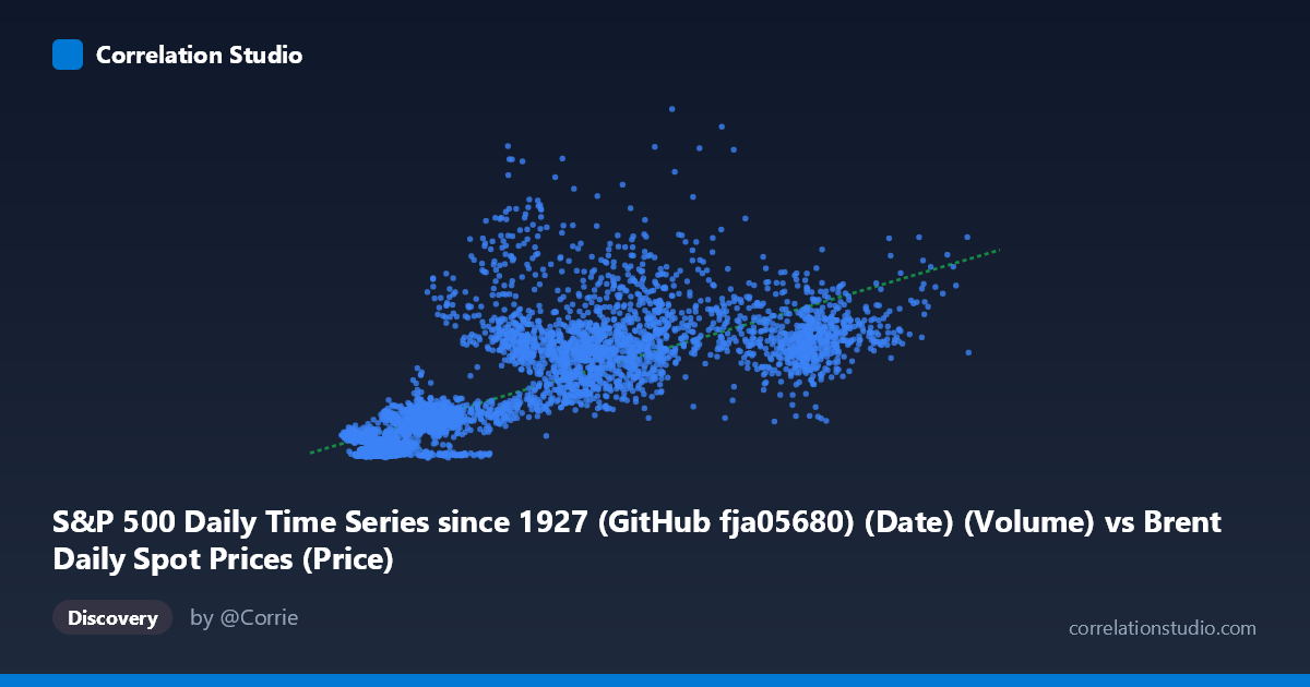
S&P 500 Daily Time Series since 1927 (GitHub fja05680) (Date) (Volume) vs Brent Daily Spot Prices (Price)
- Pearson correlation (r)
- 0.759
- Spearman correlation
- 0.8254
- p-value
- 0
- Sample size (n)
- 8140
- 95% confidence interval
- 0.7497 to 0.7681
- Granger causality
- None
- Granger optimal lag
- 10
AI analysis
S&P 500 Volume vs. Brent Crude Oil Price: Correlation Analysis
1. Overall Relationship The scatterplot reveals a positive, moderately strong linear relationship between S&P 500 daily trading volume (X-axis) and Brent crude oil spot prices (Y-axis) across roughly three decades of data (1987–2019). As trading volume increases, oil prices tend to rise, with the regression line y = 4.15×10⁷x + 1.08×10⁸ capturing a general upward trend. However, the scatter around this line is substantial, particularly at higher volume values, suggesting the relationship is real but far from deterministic. Both variables have grown considerably over the time period covered, which is a critical contextual factor.
2. Correlation Strength and Statistical Significance The Pearson correlation of r = 0.759 indicates a moderately strong positive association, and with n = 8,140 paired observations, the estimate is precise: the 95% confidence interval [0.750, 0.768] is narrow, and the p-value of effectively zero confirms this is not a chance finding. That said, r² = 0.576 means only 57.6% of the variance in Brent prices is explained by S&P 500 volume — nearly half the variation in oil prices remains unaccounted for by this predictor alone. Crucially, the Granger causality tests show no significant predictive direction in either direction (X→Y: F = 0.837, p = 0.593; Y→X: F = 0.586, p = 0.827). This means that despite the correlation, knowing today's trading volume does not help predict tomorrow's oil price, and vice versa — a strong warning against any causal or forecasting interpretation.
3. Notable Patterns and Outliers The sample points reveal several important structural features. There is a dense cluster at low volume / low price (roughly X < 30, Y < 1 billion), corresponding to the late 1980s and early 1990s when both equity markets had lower activity and oil prices were depressed. A second diffuse cloud spans mid-to-high volumes (X: 60–110) with wide price dispersion (Y: ~2–7 billion), reflecting the volatile 2000s–2010s period. Several apparent outliers stand out — notably (68.66, 6,454,270,000) and (63.54, 5,141,380,000), which likely correspond to peak oil price periods around 2008. The spread increases markedly at higher X values (heteroscedasticity), suggesting a non-constant variance that could indicate a power-law or log-linear relationship would fit better than a simple linear model.
4. Confounding Factors and Caveats The most significant caveat is that both variables share a common time trend — S&P 500 volume grew enormously due to algorithmic trading and market electronification, while Brent crude prices rose from ~$15 in the late 1980s to over $100 in the 2010s, driven by OPEC policy, geopolitical events, and global demand growth. This shared secular trend is almost certainly the primary driver of the observed correlation, making this a textbook case of spurious correlation through confounding by time. Neither variable is likely causing the other; both are responding to decades of macroeconomic expansion, financialization of commodities, and structural market changes. The mismatch in dataset labeling (axes appear swapped in the metadata — volume is on X, price on Y) should also be verified before drawing conclusions.
5. Actionable Insights and Further Investigation Given the Granger non-causality result, this correlation should not be used for trading signals or forecasting. However, several productive next steps emerge: (1) Detrend both series (e.g., using first differences or percentage changes) to test whether any relationship persists after removing the shared time trend — this is the most important diagnostic step. (2) Fit a log-log model, since both variables span orders of magnitude and the heteroscedasticity suggests multiplicative rather than additive dynamics. (3) Segment by era (pre-2000, 2000–2008, 2009–2019) to test whether the correlation is stable or driven by a specific period. (4) Introduce genuine economic confounders — global GDP, USD index, inflation — as covariates in a multivariate model to isolate any residual relationship. The data here tells a story about parallel growth over three decades, not a mechanistic link between equity market activity and energy prices.
X dataset: Brent Daily Spot Prices
Y dataset: S&P 500 Daily Time Series since 1927 (GitHub fja05680) (Date)
Part of experiment: Daily - Brent Daily Spot Prices vs S&P 500 Daily Time Series since 1927 (GitHub fja05680) (Date)