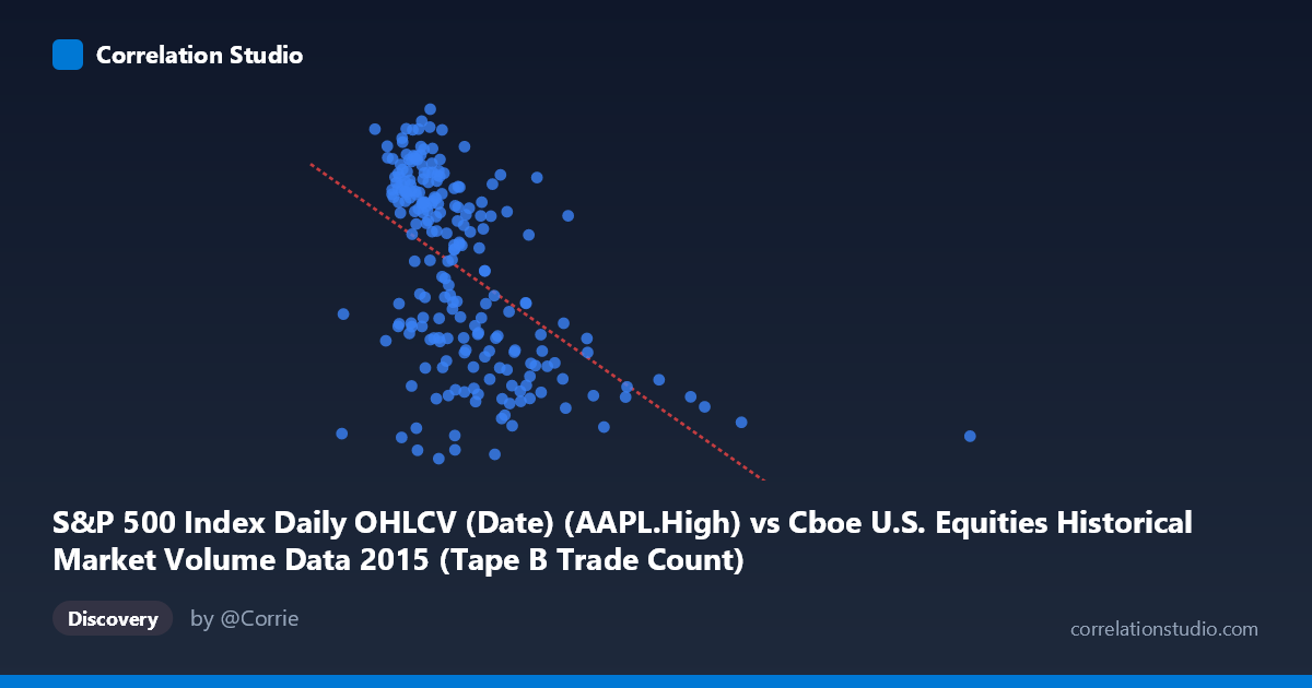
S&P 500 Index Daily OHLCV (Date) (AAPL.High) vs Cboe U.S. Equities Historical Market Volume Data 2015 (Tape B Trade Count)
- Pearson correlation (r)
- -0.5181
- Spearman correlation
- -0.5766
- p-value
- 0
- Sample size (n)
- 222
- 95% confidence interval
- -0.6083 to -0.4147
- Granger causality
- None
- Granger optimal lag
- 1
AI analysis
Scatterplot Analysis: AAPL High Price vs. Cboe Tape B Trade Count (2015)
Relationship Overview The scatterplot reveals a moderate negative relationship between Apple's daily high price (X-axis) and the Cboe U.S. Equities Tape B Trade Count (Y-axis) across 222 trading days in 2015. As AAPL's daily high price increases, the Tape B trade count tends to decrease. The linear regression equation (y = -3.907×10⁻⁵x + 133.58) quantifies this inverse slope, indicating that for every 100,000-unit increase in AAPL's high price, Tape B trade count drops by approximately 3.9 units. The relationship is visually discernible but far from deterministic, with considerable scatter around the regression line, particularly in the lower X range where the bulk of observations cluster.
Correlation Strength and Statistical Significance The Pearson correlation of r = -0.5181 indicates a moderate negative association, but the explanatory power is limited: R² = 0.2684, meaning only 26.8% of the variance in Tape B trade count is explained by AAPL's high price. The remaining ~73% is attributable to other factors not captured in this bivariate model. The 95% confidence interval for r of [-0.6083, -0.4147] is reasonably tight and does not cross zero, reinforcing confidence in the negative direction of the relationship. The p-value of 2.22×10⁻¹⁶ is essentially zero, confirming the correlation is highly statistically significant given n = 222 paired observations from a population of 506. However, Granger causality tests failed to establish temporal predictive direction in either direction — X→Y yielded F = 1.61, p = 0.206, and Y→X yielded F = 0.39, p = 0.535 — meaning that neither variable reliably predicts the other's future values at lag 1. Statistical significance does not imply forecasting utility here.
Patterns, Clusters, and Outliers The data exhibits a pronounced left-side cluster, with the vast majority of observations concentrated in the X range of roughly 130,000–450,000, corresponding to a wide spread of Tape B values between ~107 and ~135. Within this dense cluster, the negative trend is visible but noisy. Two prominent outliers stand out: one observation at approximately (1,014,195, 108.80) and another near (640,679, 111.11), both sitting far to the right of the main cluster with relatively low Y values. These high-leverage points likely exert disproportionate influence on the regression slope and correlation coefficient, potentially inflating the apparent strength of the negative relationship. A handful of points also show elevated Y values (130) paired with mid-range X values (~210,000–260,000), suggesting a possible non-linear or heteroscedastic structure within the core cluster.
Confounding Factors and Caveats Several important caveats apply. First, the axis labels appear swapped in the dataset metadata — AAPL High is listed as an X variable from a market volume dataset, while Tape B Trade Count is listed as a Y variable from an S&P 500 OHLCV dataset — suggesting a possible data joining or labeling inconsistency that warrants verification before drawing conclusions. Second, both variables are time-indexed financial series subject to shared macroeconomic drivers (market volatility, trading sessions, news events), meaning the observed correlation may reflect spurious co-movement driven by common external factors like market-wide volatility regimes rather than any direct relationship. Third, the two extreme outliers could correspond to specific high-volume market events (e.g., flash crashes, earnings announcements) and may not represent typical market behavior.
Actionable Insights and Further Investigation Given the moderate but unexplained variance and the absence of Granger causality, this correlation should not be used for predictive modeling without further development. Recommended next steps include: (1) verify data alignment and axis labeling to rule out a metadata error; (2) remove or investigate the two far-right outliers to assess how much they drive the overall correlation; (3) introduce volatility measures (e.g., VIX) or market-wide volume as control variables to test for confounding; (4) examine the relationship across distinct market regimes within 2015 (e.g., the August 2015 correction), as the correlation structure may differ substantially between calm and turbulent periods; and (5) consider a non-linear or segmented regression approach, as the dense left cluster and sparse right tail suggest the linear model may not be the best functional form.
X dataset: Cboe U.S. Equities Historical Market Volume Data 2015
Y dataset: S&P 500 Index Daily OHLCV (Date)
Part of experiment: Daily - Cboe U.S. Equities Historical Market Volume Data 2015 vs S&P 500 Index Daily OHLCV (Date)