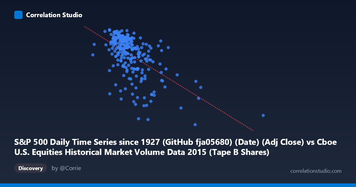
S&P 500 Daily Time Series since 1927 (GitHub fja05680) (Date) (Adj Close) vs Cboe U.S. Equities Historical Market Volume Data 2015 (Tape B Shares)

Pearson correlation (r): -0.5686
Spearman correlation: -0.5448
p-value: 0
Sample size (n): 252
95% confidence interval: -0.6467 to -0.4786
Granger causality: None
Granger optimal lag: 7

AI analysis

Analysis: S&P 500 Adjusted Close vs. Cboe Tape B Share Volume (2015)

Relationship Overview The scatterplot reveals a negative relationship between S&P 500 adjusted closing prices and Cboe Tape B share volumes during 2015. As the S&P 500 price level increases, Tape B share volume tends to decrease, and conversely, lower price levels are associated with higher trading volumes. This is a well-recognized phenomenon in equity markets — periods of market stress and price declines typically generate elevated trading activity as investors react to volatility, rebalance portfolios, or capitulate. The linear regression equation (y = -1.09×10⁻⁶x + 2173.78) quantifies this inverse slope, though the relationship is clearly not tight, with substantial scatter around the fitted line.

Correlation Strength and Statistical Significance The Pearson correlation of r = -0.5686 indicates a moderate negative association. The r² of 0.3233 means that approximately 32.3% of the variance in Tape B share volume is explained by the S&P 500 price level — meaningful, but leaving roughly 68% of variability unexplained by this relationship alone. The 95% confidence interval of [-0.6467, -0.4786] is entirely negative and relatively narrow given the sample size of 252 paired observations drawn from a population of 3,302, and the p-value of essentially 0 confirms this is highly statistically significant — chance is an implausible explanation. However, Granger causality tests tell a more nuanced story: neither direction (X→Y nor Y→X) reaches significance at conventional thresholds (F = 1.90, p = 0.070 for X→Y; F = 0.52, p = 0.818 for Y→X). This means that while a contemporaneous correlation exists, past S&P 500 prices do not reliably predict future Tape B volumes, and vice versa — the relationship may be driven by simultaneous common factors rather than any directional lead-lag dynamic.

Patterns, Clusters, and Outliers Several features stand out in the data. The bulk of observations cluster in the S&P 500 range of roughly 70M–130M (in the scaled X-axis units representing dates/price levels), with Tape B volumes concentrated between approximately 2,040 and 2,130. There are notable outliers in the lower-right region — points such as (205,030,139; 1867.61) and (130,951,901; 1881.77) represent episodes of significantly depressed prices coinciding with elevated volume, consistent with the August 2015 market correction. Conversely, the upper-left cluster shows elevated prices with more moderate volumes during quieter stretches of 2015. The spread widens noticeably at lower price levels, suggesting heteroscedasticity — volume becomes more variable precisely when markets are most stressed, which is practically important for risk modeling.

Confounding Factors and Caveats Several important caveats apply. First, the X-axis encodes calendar date-indexed price, meaning time itself is embedded in the variable — secular trends in 2015 (bull market early in the year, August correction, partial recovery) may be driving what appears to be a price-volume relationship but is partly a temporal trend artifact. Second, Tape B specifically covers NYSE American (AMEX) and regional exchange securities, not the full market, so it may respond to sector-specific dynamics not captured by the broad S&P 500 index. Third, market structure changes — such as shifts in algorithmic trading activity, ETF rebalancing cycles, or options expiration dates — could generate volume spikes independent of price levels. Finally, the failure of Granger causality to achieve significance (X→Y p = 0.070 is borderline) at the chosen lag of 7 periods may be sensitive to lag selection, and a marginally different specification could alter conclusions.

Actionable Insights and Further Investigation Practitioners should avoid treating this correlation as a predictive tool given the absence of confirmed Granger causality — the relationship is associative, not demonstrably directional. For further investigation, it would be valuable to: (1) decompose the time series to separate trend from cyclical components before correlating, removing the date-as-confounder issue; (2) test whether implied volatility (VIX) acts as a mediating variable explaining both lower prices and higher volumes simultaneously; (3) examine nonlinear or regime-switching models, as the heteroscedasticity suggests the relationship may behave differently in high- versus low-volatility regimes; and (4) expand the analysis across multiple years to test whether the 2015 relationship (heavily influenced by the August correction) generalizes or is period-specific. The ~68% unexplained variance is a clear invitation to incorporate additional predictors such as VIX, sector flows, or macroeconomic surprise indices.

X dataset: Cboe U.S. Equities Historical Market Volume Data 2015

Y dataset: S&P 500 Daily Time Series since 1927 (GitHub fja05680) (Date)

Part of experiment: Daily - Cboe U.S. Equities Historical Market Volume Data 2015 vs S&P 500 Daily Time Series since 1927 (GitHub fja05680) (Date)