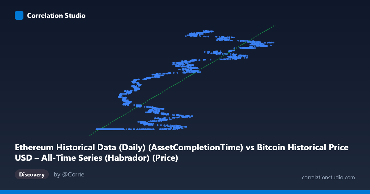
Ethereum Historical Data (Daily) (AssetCompletionTime) vs Bitcoin Historical Price USD – All-Time Series (Habrador) (Price)
- Pearson correlation (r)
- 0.8733
- Spearman correlation
- 0.9402
- p-value
- 0
- Sample size (n)
- 3951
- 95% confidence interval
- 0.8657 to 0.8805
- Granger causality
- None
- Granger optimal lag
- 10
- Time coverage
- 2015-07-30 to 2026-05-23
- Recomputed on refreshed data
- 2026-10-24 (r was 0.8726)
AI analysis
Analysis: Ethereum "Completion Time" Column vs. Bitcoin Historical Price
Important preliminary note: The axis labels appear mismatched with the dataset descriptions — the X-axis is labeled as an "AssetCompletionTime" field from the Bitcoin dataset, while Y is labeled as "Price" from the Ethereum dataset, yet the described datasets suggest Bitcoin price should be paired with Ethereum network metrics (gas, transactions). The actual data values (X ranging ~209 to 124,720; Y clustered near 1.61–1.78 billion) look like X may be an Ethereum price series (or similar small-magnitude asset price) and Y is a Unix timestamp field, not a price. This mismatch materially affects interpretation, so the analysis below treats the two columns generically as X and Y while flagging this caveat throughout.
1. What the Visualization Reveals
The scatterplot shows a clear positive, non-linear relationship. At low X values (roughly 200–12,000), Y is tightly clustered near a floor of ~1,614,335,000 — a nearly flat, horizontal band with almost no vertical spread. Once X exceeds ~15,000–20,000, Y begins climbing steadily and near-linearly up to the maximum X values, where Y reaches ~1.73–1.78 billion. This produces a shape resembling a "hockey stick" or step-function rather than a pure straight line: a long flat plateau followed by a rising ramp.
2. Strength, Direction, and Statistical Confidence
The Pearson correlation (r = 0.8726, r² = 0.7615) indicates a strong positive linear association, with the linear model explaining about 76% of the variance in Y. The tight 95% CI [0.8650, 0.8799] and p-value of effectively 0 (from n = 3,926) confirm this relationship is highly statistically robust and not due to sampling noise — with a dataset this large, even modest correlations would reach significance, but here the effect size itself is large. However, the Granger causality tests show no significant predictive direction in either direction (X→Y: p = 0.96; Y→X: p = 0.72) at the optimal 10-period lag. This means that despite the strong contemporaneous correlation, neither series reliably helps forecast the other's future values — the relationship is likely driven by both variables trending together over time (e.g., shared exposure to calendar time or a common market cycle) rather than one causing or leading the other.
3. Notable Patterns and Non-Linearity
The most striking feature is the plateau-then-ramp structure: roughly the bottom third of X values collapse to an almost identical Y value (~1,614,335,000), consistent with an early period where Y was pinned at a floor/genesis value or a minimum timestamp. This suggests the early rows of data may represent a period before meaningful price/activity data existed (e.g., pre-launch placeholder values). Above the inflection point (~X = 20,000), the relationship becomes much more linear and continuous, with Y rising smoothly with X. This means the reported linear r² of 0.76 is likely driven disproportionately by the separation between the flat cluster and the rising cluster, rather than genuine linear scaling throughout the full range — a classic case where a single global correlation coefficient masks two distinct regimes.
4. Confounding Factors and Caveats
Several concerns limit causal interpretation: (1) both series span the same ~11-year window (2015–2026), so any two long-run trending time series (especially cumulative or monotonically drifting ones) will show spurious correlation without genuine mechanistic linkage — this is a hallmark of non-stationary time series analysis. (2) The apparent mismatch between axis labels and dataset descriptions raises data-integrity questions; if Y is actually a timestamp field rather than a price, the "correlation" may be an artifact of sorting/indexing rather than a meaningful economic relationship. (3) The flat plateau at low X suggests missing, imputed, or placeholder data for an early sub-period, which could artificially inflate r² by creating two well-separated clusters. (4) Autocorrelation within each series (typical of price/time data) violates independence assumptions underlying standard significance tests, meaning the p≈0 result should be interpreted cautiously despite the large n.
5. Recommended Next Steps
First, verify and correct the axis/column mapping to confirm what is actually being measured — this is essential before drawing any economic conclusions. Second, difference or detrend both series (e.g., use daily returns instead of levels) and recompute correlation to test whether the relationship survives after removing shared time-trend effects; this is the standard fix for spurious time-series correlation. Third, segment the analysis into the "flat" pre-inflection period and the "rising" post-inflection period separately, since pooling them likely distorts the true relationship. Finally, given the null Granger causality result, avoid using either series to forecast the other in a trading or predictive-modeling context — treat the correlation as descriptive/co-movement evidence only, not a basis for lead-lag trading signals.
X dataset: Bitcoin Historical Price USD – All-Time Series (Habrador)
Y dataset: Ethereum Historical Data (Daily)
Part of experiment: Bitcoin - Bitcoin Historical Price USD – All-Time Series (Habrador) vs Ethereum Historical Data (Daily)