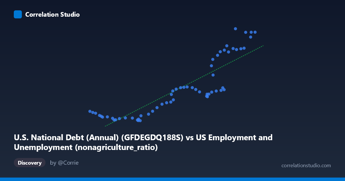
U.S. National Debt (Annual) (GFDEGDQ188S) vs US Employment and Unemployment (nonagriculture_ratio)
- Pearson correlation (r)
- 0.8725
- Spearman correlation
- 0.9037
- p-value
- 0
- Sample size (n)
- 60
- 95% confidence interval
- 0.7946 to 0.9221
- Granger causality
- None
- Granger optimal lag
- 10
AI analysis
Analysis: U.S. National Debt vs. Non-Agriculture Employment Ratio
Relationship Overview
The scatterplot reveals a clear, positive relationship between U.S. National Debt (as a percent of GDP) and the non-agriculture employment ratio across the 1966–2025 time period. As national debt rises, the non-agriculture employment ratio tends to increase as well. The linear regression equation (y = 0.000924x − 46.38) confirms this upward trend, though the data visibly clusters into at least two distinct behavioral zones rather than forming a single, uniform cloud — suggesting the relationship is not entirely linear and may reflect different economic regimes across the six-decade span.
Correlation Strength and Statistical Significance
The correlation is strong and statistically robust: r = 0.8725, with r² = 0.7612, meaning approximately 76.1% of the variance in the non-agriculture employment ratio is explained by national debt levels. This is a meaningfully high explanatory share for macroeconomic data. The 95% confidence interval for r is [0.7946, 0.9221], which is relatively tight and excludes zero by a wide margin, and the p-value is effectively zero, confirming this is not a chance association across the n = 60 paired observations. However, the Granger causality tests complicate any causal interpretation: neither direction (X→Y: F = 0.852, p = 0.586; Y→X: F = 1.563, p = 0.168) reaches significance at conventional thresholds, even with an optimal lag of 10 periods. This means that while the two variables move together strongly, neither reliably predicts the other's future values in a temporal sense — a critical caveat against assuming debt "drives" employment structure or vice versa.
Notable Patterns, Clusters, and Non-Linearity
Two distinct clusters are visually apparent. The first groups observations roughly in the lower-left (debt ~68,000–110,000; ratio ~30–50), corresponding largely to earlier decades when debt-to-GDP was lower and non-agriculture employment shares were smaller. The second cluster occupies the upper-right (debt ~130,000–161,000; ratio ~55–124), representing more recent periods of elevated federal debt and higher non-agriculture ratios. Within this upper cluster, there is notable vertical spread — several points around debt levels of 135,000–148,000 span ratios from ~57 to ~107, suggesting that at similar debt levels, employment ratios vary substantially. Points like (150,290; 124.04) and (161,268; 120.55) appear as potential high-leverage outliers at the upper extreme, while (68,915; 40.34) anchors the lower bound. This spread implies a possible non-linear or threshold effect, where the relationship steepens at higher debt levels or where a third variable introduces dispersion.
Confounding Factors and Caveats
This correlation almost certainly reflects shared secular trends rather than a direct causal mechanism. Both variables have been driven upward over decades by structural forces: deindustrialization increasing non-agriculture employment shares, demographic shifts, globalization, and successive fiscal expansions (especially post-2008 and post-2020). The absence of Granger causality at a 10-period lag reinforces that these are co-trending time series — a classic source of spurious or inflated correlations. Omitted variables such as GDP growth cycles, interest rate regimes, labor force composition changes, and major fiscal events (New Deal legacy, Reagan-era debt expansion, COVID-19 stimulus) almost certainly mediate or confound the observed relationship. Additionally, using annual aggregates masks within-year volatility and may smooth over recession-recovery dynamics that would alter the picture.
Actionable Insights and Further Investigation
Given the strong co-movement but absent Granger causality, the priority for further investigation should be detrending both series (e.g., via first-differencing or HP filtering) to test whether the correlation persists beyond shared long-run trends — a finding of near-zero residual correlation would confirm the relationship is largely spurious. Researchers should also explore regime-segmented analysis, splitting the sample at structural breakpoints (e.g., 1980, 2008, 2020) to determine whether the debt–employment relationship strengthens or reverses within distinct fiscal eras. Including mediating variables such as real GDP growth, the unemployment rate, and interest expenditure as share of GDP in a multivariate model would clarify whether debt carries independent explanatory power. Finally, examining non-linear specifications (quadratic or piecewise regression) may better capture the apparent threshold behavior visible in the upper-right cluster and improve out-of-sample forecasting utility.
X dataset: US Employment and Unemployment
Y dataset: U.S. National Debt (Annual)
Part of experiment: Yearly - US Employment and Unemployment vs U.S. National Debt (Annual)