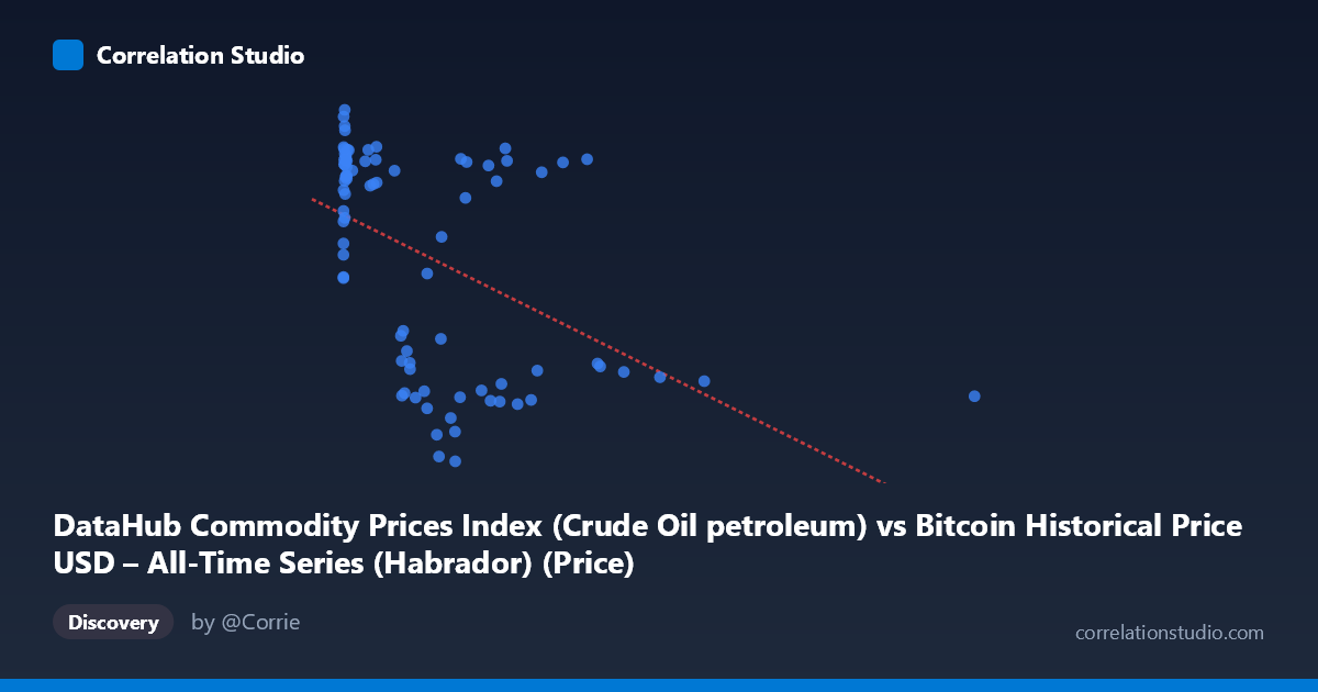
DataHub Commodity Prices Index (Crude Oil petroleum) vs Bitcoin Historical Price USD – All-Time Series (Habrador) (Price)
- Pearson correlation (r)
- -0.4792
- Spearman correlation
- -0.4719
- p-value
- 0.000005
- Sample size (n)
- 83
- 95% confidence interval
- -0.6298 to -0.2938
- Granger causality
- None
- Granger optimal lag
- 8
- Time coverage
- 2010-08-01 to 2017-06-01
- Recomputed on refreshed data
- 2026-10-24 (r was -0.4792)
AI analysis
Analysis: Bitcoin Price vs. Commodity Price Index
1. Overview of the Relationship
The scatterplot displays a negative, moderately weak relationship between Bitcoin's historical USD price (X-axis) and a commodity price index (Y-axis, covering crude oil and broader commodities). Despite the labeling suggesting a temporal pairing, this is fundamentally a cross-variable comparison across 83 sampled points spanning 2010–2017. The data shows a distinctive pattern: a dense cluster of points at low X-values (Bitcoin under ~50 USD) with commodity index values ranging broadly from ~140 to 220, followed by a sparser scatter of points at higher Bitcoin prices (200–2450) where commodity values compress into a lower band (~56–200).
2. Strength, Direction, and Statistical Confidence
The correlation coefficient (r = -0.479) indicates a moderate negative relationship, with r² = 0.230 meaning only about 23% of the variance in commodity prices is explained by Bitcoin price movements (or vice versa) — leaving roughly 77% of variance attributable to other factors. The 95% confidence interval [-0.630, -0.294] is reasonably tight and entirely negative, and the p-value (4.6 × 10⁻⁶) is highly significant, giving strong confidence that a real negative association exists rather than being a sampling artifact. However, statistical significance should not be conflated with practical predictive power — the modest r² means this relationship alone is a weak basis for forecasting one variable from the other. Critically, the Granger causality tests (both directions non-significant, p = 0.249 and p = 0.167) indicate neither variable helps predict the other's future values in a time-series sense. This suggests the correlation is likely driven by both series independently trending over the same historical period rather than genuine causal or lead-lag dynamics.
3. Notable Patterns and Outliers
The chart reveals a distinctly non-linear, almost bifurcated structure rather than a clean linear trend. Low Bitcoin-price points (X < 50) show high variance in Y (140–222), representing Bitcoin's early years (2010–2012) when commodity prices were elevated post-financial-crisis. As Bitcoin prices climb into the hundreds and thousands (later years, 2014–2017), commodity index values cluster lower (56–103) with a few exceptions (points like 629.02, 203.83 or 946.92, 198.69 breaking this pattern). This creates two loosely separated point-clouds rather than a continuous negative slope, suggesting the relationship is largely an artifact of two independent secular trends (Bitcoin rising, commodities falling/recovering) overlapping in calendar time rather than true bivariate dependence. The linear fit (R²=0.230) likely overstates the "fit quality" given this clustering behavior.
4. Confounding Factors and Caveats
The most significant caveat is that this is a time-series confound: both Bitcoin's price and commodity indices have their own trends, cycles, and macroeconomic drivers (monetary policy, oil supply shocks, USD strength, speculative bubbles) that coincidentally moved in opposite directions during 2010–2017. Correlating two trending time series without detrending or differencing frequently produces spurious correlation — a classic econometric pitfall. The lack of Granger causality reinforces that this is likely a spurious or trend-driven correlation rather than a functional relationship. Additionally, the extreme skew in X (range 0.06 to 2452, mean 321, but heavily right-tailed) means a few high-leverage points (e.g., X=2452.18) could disproportionately influence both r and the regression slope.
5. Recommendations for Further Investigation
To validate whether any genuine relationship exists, analysts should: (1) detrend or difference both series (e.g., use returns/percent changes rather than levels) before correlating, which typically eliminates spurious trend-driven correlations; (2) test for cointegration rather than simple correlation, given both are non-stationary price series; (3) examine sub-periods separately (pre-2013 vs. post-2013) since the bifurcated cluster pattern suggests structural change; and (4) incorporate known macro confounders (USD index, interest rates, oil supply events) as control variables. Given the non-significant Granger results, this pairing should not be used for predictive trading models linking Bitcoin and commodity prices in either direction.
X dataset: Bitcoin Historical Price USD – All-Time Series (Habrador)
Y dataset: DataHub Commodity Prices Index
Part of experiment: Bitcoin - Bitcoin Historical Price USD – All-Time Series (Habrador) vs DataHub Commodity Prices Index