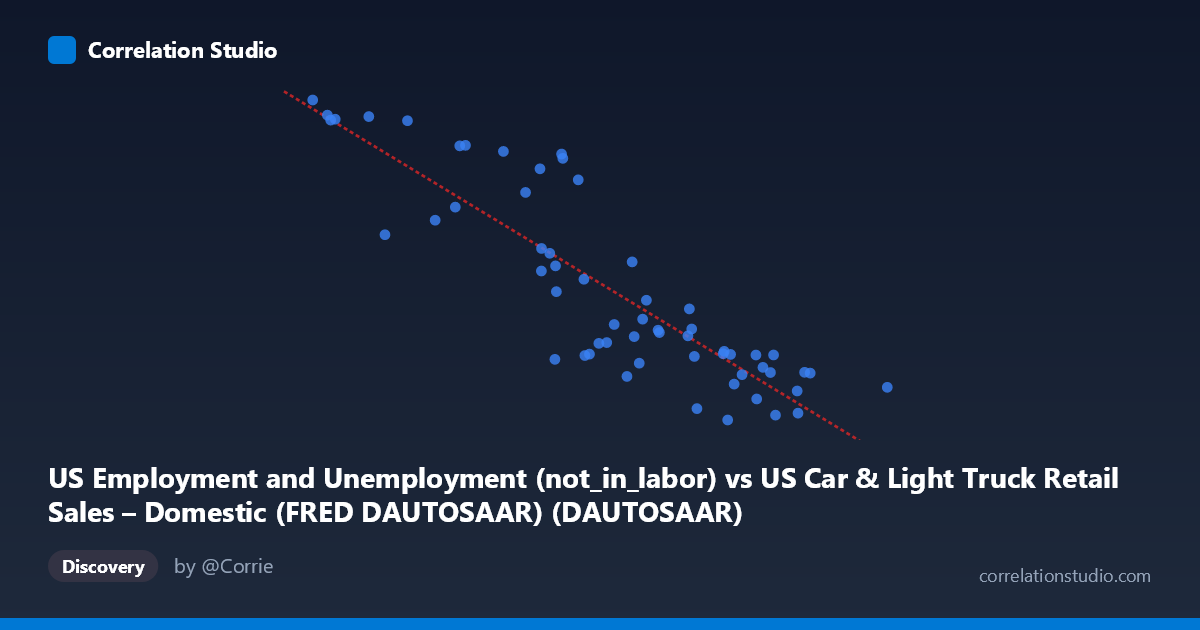
US Employment and Unemployment (not_in_labor) vs US Car & Light Truck Retail Sales – Domestic (FRED DAUTOSAAR) (DAUTOSAAR)
- Pearson correlation (r)
- -0.8754
- Spearman correlation
- -0.8756
- p-value
- 0
- Sample size (n)
- 59
- 95% confidence interval
- -0.9243 to -0.7982
- Granger causality
- None
- Granger optimal lag
- 10
AI analysis
Analysis: US Not-in-Labor-Force vs. Domestic Auto Retail Sales
1. Relationship Overview The scatterplot reveals a clear negative linear relationship between the number of Americans not in the labor force (X-axis) and domestic auto retail sales (Y-axis, DAUTOSAAR). As the not-in-labor-force population increases, domestic auto sales decline in a consistent, structured pattern. The linear regression equation (y = -6,624x + 113,765) confirms this inverse slope, suggesting that for each unit increase in the not-in-labor-force measure, auto sales decrease by approximately 6,624 units (annualized rate). The data spans nearly six decades (1967–2025), giving the relationship substantial temporal breadth and historical credibility.
2. Correlation Strength, Direction, and Causality The correlation coefficient of r = -0.8754 indicates a strong negative association, and the R² of 0.7663 means that approximately 76.6% of the variance in domestic auto sales is statistically explained by variation in the not-in-labor-force measure — a remarkably high explanatory share for a single-variable model in macroeconomic data. The 95% confidence interval of [-0.9243, -0.7982] is narrow and entirely negative, reinforcing high confidence in the direction and magnitude of the association. The p-value of effectively zero confirms this is not a chance finding at any conventional significance threshold. However, Granger causality tests reveal no significant predictive directionality in either direction (X→Y: F=0.97, p=0.49; Y→X: F=0.99, p=0.47), even at the optimal lag of 10 periods. This is a critical caveat: despite the strong correlation, neither variable reliably leads or predicts the other temporally, strongly suggesting that both are being driven by common underlying forces rather than one causing the other.
3. Notable Patterns, Clusters, and Outliers The data clusters loosely into two regions: a high-sales / low not-in-labor-force cluster (X ≈ 2–5, Y ≈ 80,000–103,000) and a lower-sales / higher not-in-labor-force cluster (X ≈ 7–10, Y ≈ 52,000–70,000). Several observations warrant attention. Points near (2.07–2.18, 99,826–100,465) represent extreme high-sales, low not-in-labor-force conditions — likely reflecting peak mid-cycle economic expansions from earlier decades. Conversely, (10.14, 57,667) and (8.85, 53,602) anchor the lower-right extreme. A few notable outliers from the linear trend exist in the mid-range: (5.46, 93,671), (5.68, 90,290), and (5.44, 94,351) show much higher-than-predicted auto sales for their X values, suggesting episodic demand spikes (e.g., post-recession pent-up demand or incentive-driven buying). There is also mild heteroscedasticity — residual spread appears slightly larger at lower X values, hinting that the linear model may underfit the upper-left region.
4. Confounding Factors and Interpretive Caveats The most important caveat is that both variables are strongly co-determined by the macroeconomic cycle. The not-in-labor-force population grows during recessions and demographic aging, while auto sales collapse during the same periods — creating a spurious-looking causal relationship. The secular aging of the US population is a major structural confound: as Baby Boomers retire, not-in-labor-force numbers rise mechanically, independent of economic conditions. Additionally, auto sales are influenced by interest rates, credit availability, fuel prices, and consumer confidence — none of which are controlled for here. The Granger non-causality result reinforces that this correlation is likely spurious or confounded, driven by shared long-run trends (demographic shifts, business cycles) rather than any direct mechanism. The 10-period optimal lag with non-significant results also suggests that short- to medium-term dynamics don't align between these two series.
5. Actionable Insights and Further Investigation Given the strong but likely spurious correlation, analysts should not use not-in-labor-force counts as a direct predictor of auto sales in forecasting models without controlling for confounders. Recommended next steps include: (1) decomposing the not-in-labor-force variable into retirement-driven vs. discouraged-worker components to isolate demand-relevant signals; (2) introducing co-variates such as consumer credit conditions, the unemployment rate, and real disposable income to partial out shared cycle effects; (3) applying cointegration testing (e.g., Engle-Granger or Johansen) to determine whether a genuine long-run structural relationship exists, as both series appear non-stationary; and (4) examining the mid-range outliers (Y values ~90,000+ at X ≈ 5.4–5.7) as potential regime-change episodes worth modeling separately. A VAR model incorporating GDP growth and interest rates would likely reveal that the apparent X–Y relationship dissolves substantially once macroeconomic context is accounted for.
X dataset: US Car & Light Truck Retail Sales – Domestic (FRED DAUTOSAAR)
Y dataset: US Employment and Unemployment
Part of experiment: Yearly - US Car & Light Truck Retail Sales – Domestic (FRED DAUTOSAAR) vs US Employment and Unemployment