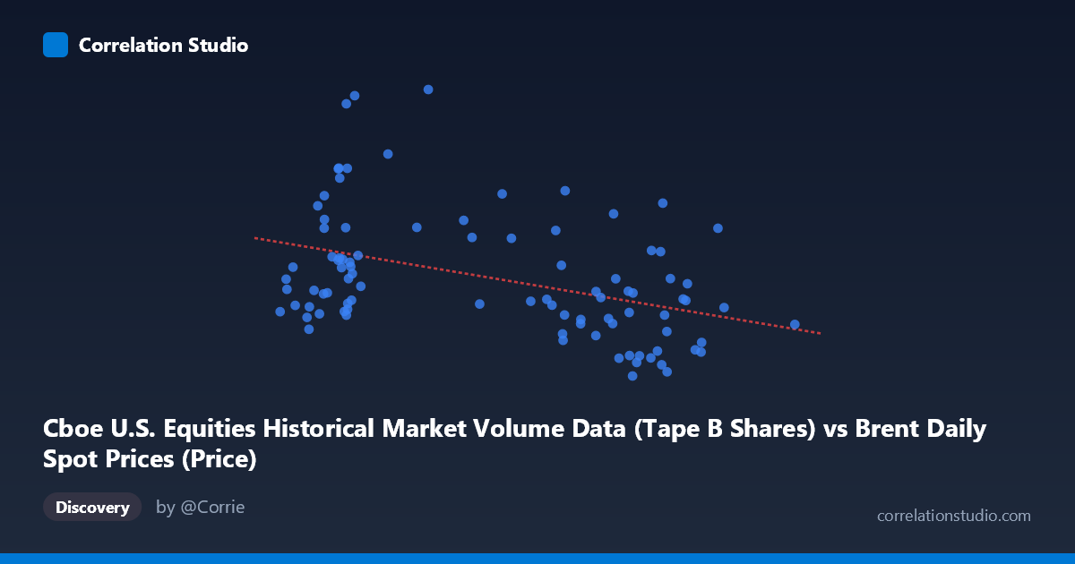
Cboe U.S. Equities Historical Market Volume Data (Tape B Shares) vs Brent Daily Spot Prices (Price)
- Pearson correlation (r)
- -0.4122
- Spearman correlation
- -0.3863
- p-value
- 0.000044
- Sample size (n)
- 92
- 95% confidence interval
- -0.569 to -0.2266
- Granger causality
- None
- Granger optimal lag
- 10
AI analysis
Analysis: Brent Crude Oil Prices vs. Cboe Tape B Equity Market Volume
1. Overall Relationship The scatterplot reveals a moderate negative relationship between Europe Brent crude oil spot prices (X-axis, USD/barrel) and Cboe Tape B U.S. equity market share volume (Y-axis). As crude oil prices increase, equity market volume on Tape B exchanges tends to decline. The linear regression equation (y = -1,006,920x + 317,974,000) quantifies this: each additional dollar per barrel in Brent crude is associated with approximately 1 million fewer Tape B shares traded. The relationship is visible but noisy, with considerable scatter around the regression line, suggesting that while the trend exists, it is far from deterministic.
2. Correlation Strength, Direction, and Causality The Pearson correlation of r = -0.41 indicates a moderate negative association. However, the coefficient of determination r² = 0.17 is critical context: only 17% of the variance in Tape B equity volume is statistically explained by Brent crude prices, meaning roughly 83% of volume fluctuations are driven by other factors entirely. The p-value of 4.44 × 10⁻⁵ confirms the correlation is highly statistically significant and very unlikely to be a chance finding, while the 95% confidence interval of [-0.57, -0.23] confirms the negative direction is robust but acknowledges meaningful uncertainty in the magnitude. Importantly, Granger causality tests in both directions are non-significant (X→Y: p = 0.59; Y→X: p = 0.77), meaning neither variable reliably predicts the other temporally with up to a 10-period lag. This rules out a straightforward predictive or lead-lag trading relationship and suggests any correlation is likely contemporaneous or driven by shared external forces.
3. Notable Patterns, Clusters, and Outliers Several features stand out in the data. There is a visible cluster of high-volume observations at lower oil prices (roughly X = 61–75 USD/barrel, Y = 190–390 million shares), which drives much of the negative slope. A few prominent outliers warrant attention: the point at approximately (83.28, 393,280,831) represents an unusually high volume day at a moderate oil price, and multiple observations near (71–72, 320–387 million) cluster at elevated volumes well above the regression line. At higher oil prices (X 110), volume values are more tightly compressed in the 136–290 million range, suggesting reduced dispersion at higher price levels. The data also hints at possible non-linearity: volume appears to drop sharply as oil moves from ~65 to ~100 USD/barrel, but the relationship flattens somewhat above 100, potentially warranting a logarithmic or piecewise model.
4. Confounding Factors and Interpretive Caveats Several important caveats apply. First, this covers only January–May 2026, a short 4.5-month window that may reflect idiosyncratic market conditions rather than a structural relationship. Second, Tape B volume specifically covers regional exchange activity, which may be influenced by exchange routing rules, market-maker behavior, and regulatory changes unrelated to oil prices. Third, the most plausible interpretation is that both variables respond to the same macro regime: risk-off environments (geopolitical stress, recession fears) could simultaneously suppress oil demand/prices and reduce equity trading appetite, or conversely, inflationary spikes could drive oil up while dampening equity volumes. Fourth, the population N = 1,980 vs. sample n = 92 warrants attention — the broader population context suggests temporal autocorrelation is likely in the daily data, which could inflate statistical significance. Finally, dataset label mismatches (Brent price data contains a Tape B volume column and vice versa) suggest these may be joined datasets, and any join methodology errors could introduce artifacts.
5. Actionable Insights and Further Investigation Given the non-significant Granger causality, practitioners should not use Brent crude prices as a tactical predictor of next-day Tape B volume at any tested lag. However, the contemporaneous correlation suggests monitoring oil price regimes as a macro-context indicator for equity volume conditions. Several next steps are recommended: (1) Extend the time series beyond 4.5 months to test whether the relationship is structural or period-specific; (2) Test non-linear models (quadratic, log-log) given the apparent flattening at higher price levels; (3) Investigate the high-volume outlier days (e.g., ~83 USD/barrel, 393M shares) for event-driven explanations such as expiration dates, Fed announcements, or index rebalancing; (4) Control for VIX or market volatility as a potential common driver of both variables; and (5) Decompose by Tape A and C to determine whether the negative relationship is specific to Tape B or a broader equity market phenomenon.
X dataset: Brent Daily Spot Prices
Y dataset: Cboe U.S. Equities Historical Market Volume Data
Part of experiment: Daily - Brent Daily Spot Prices vs Cboe U.S. Equities Historical Market Volume Data