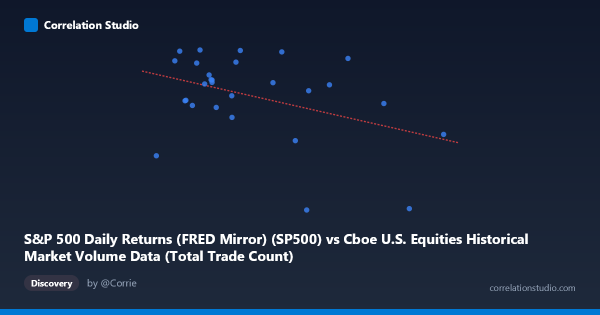
S&P 500 Daily Returns (FRED Mirror) (SP500) vs Cboe U.S. Equities Historical Market Volume Data (Total Trade Count)
- Pearson correlation (r)
- -0.4041
- Spearman correlation
- -0.2501
- p-value
- 0.032945
- Sample size (n)
- 28
- 95% confidence interval
- -0.6754 to -0.0365
- Granger causality
- None
- Granger optimal lag
- 7
AI analysis
Analysis: S&P 500 Daily Returns vs. Cboe Total Trade Count
Relationship Overview The scatterplot reveals a modest negative relationship between S&P 500 price levels (X-axis, serving as a proxy for market valuation) and total trade count on U.S. equities exchanges (Y-axis). As the S&P 500 index value increases — particularly at higher values above ~8,000,000 — trade counts tend to drift lower, suggesting that elevated market valuations may coincide with reduced trading activity. However, the distribution of points is notably scattered, and the linear trend is far from clean, with considerable dispersion across the full X range of approximately 5.7M to 9.4M.
Correlation Strength and Statistical Interpretation The Pearson correlation of r = -0.4041 indicates a weak-to-moderate negative association. Critically, R² = 0.1633, meaning only 16.3% of the variance in trade count is explained by the S&P 500 level — leaving more than 83% attributable to other factors. The 95% confidence interval for r spans [-0.6754, -0.0365], a wide range that barely excludes zero, underscoring meaningful uncertainty in the true population correlation. The p-value of 0.033 clears the conventional 0.05 threshold, suggesting the result is nominally statistically significant, though given the small sample (n = 28) and wide CI, this should be interpreted cautiously. The Granger causality analysis adds a crucial qualifier: neither direction (X→Y nor Y→X) achieves significance at the 0.05 level (p = 0.101 and p = 0.096, respectively), meaning there is no demonstrable temporal predictive relationship — higher S&P 500 values do not reliably precede changes in trade count, nor vice versa.
Notable Patterns and Outliers Several data points warrant attention. The point near (7,668,198, 6,796.86) sits conspicuously low in trade count relative to its X position, appearing as a potential downside outlier that may be disproportionately influencing the negative slope. Similarly, (8,981,120, 6,798.40) reinforces the low-trade-count pattern at high S&P 500 values. Conversely, multiple points cluster in the 6.0M–6.8M X range with trade counts near 6,940–6,978, forming a relatively dense group at moderate valuations and high activity. There is also a hint of a non-linear pattern — trade counts appear relatively stable and high across the mid-range of X, then drop more sharply at the extremes, suggesting a possible curved or threshold relationship rather than a purely linear one.
Confounding Factors and Caveats Several important caveats apply. First, the X-axis label and dataset descriptions appear inverted — the X variable is drawn from the Cboe volume dataset while the Y variable comes from the FRED S&P 500 dataset, which is an unusual axis assignment that could reflect a data pipeline error or intentional analytical framing requiring careful interpretation. Second, the time window is narrow (Jan 2–Feb 11, 2026; ~41 trading days, sampled at n=28), so seasonal effects, macro events, or a single volatility regime could dominate the signal. Third, trading volume and trade count are influenced heavily by algorithmic activity, options expiration cycles, index rebalancing, and market structure changes — all unrelated to price level directly. Finally, the population size listed as N = 1,980 versus n = 28 sampled suggests substantial under-sampling, which limits the generalizability of findings.
Actionable Insights and Further Investigation Given the weak explanatory power and absent Granger causality, practitioners should avoid using S&P 500 levels as a standalone predictor of trade count in any tactical model. More productive next steps would include: (1) extending the time series to capture multiple market regimes and improve statistical power; (2) testing non-linear models (e.g., polynomial or spline regression) given the visual hint of curvature; (3) incorporating volatility measures (e.g., VIX) as a co-variate, since volatility — not price level — is more theoretically linked to trading activity; and (4) resolving the axis/dataset labeling discrepancy to ensure the analytical direction is intentional and interpretable. A multivariate regression incorporating VIX, bid-ask spreads, and time-of-month effects would likely yield far stronger and more actionable models.
X dataset: Cboe U.S. Equities Historical Market Volume Data
Y dataset: S&P 500 Daily Returns (FRED Mirror)
Part of experiment: Daily - Cboe U.S. Equities Historical Market Volume Data vs S&P 500 Daily Returns (FRED Mirror)