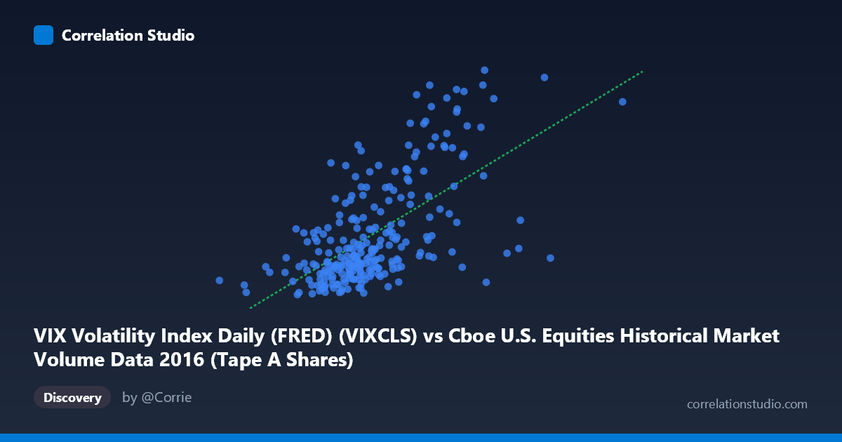
VIX Volatility Index Daily (FRED) (VIXCLS) vs Cboe U.S. Equities Historical Market Volume Data 2016 (Tape A Shares)
- Pearson correlation (r)
- 0.6184
- Spearman correlation
- 0.5889
- p-value
- 0
- Sample size (n)
- 252
- 95% confidence interval
- 0.5357 to 0.6893
- Granger causality
- None
- Granger optimal lag
- 1
AI analysis
Analysis: VIX Volatility Index vs. Cboe U.S. Equities Market Volume (Tape A Shares, 2016)
Relationship Overview
The scatterplot reveals a positive relationship between daily U.S. equity market volume (Tape A Shares, measured in notional value on the X-axis) and the VIX Volatility Index (Y-axis) across 252 trading days in 2016. The linear regression equation (y = 4.18×10⁻⁸x + 4.45) confirms this upward trend: as market volume increases, VIX tends to rise as well. This is financially intuitive — periods of elevated market fear and uncertainty (high VIX) typically coincide with surges in trading activity, as investors actively reposition portfolios in response to volatility. However, the scatterplot also shows considerable dispersion around the regression line, signaling that volume alone tells an incomplete story about VIX levels.
Correlation Strength and Statistical Interpretation
The correlation coefficient of r = 0.6184 indicates a moderate-to-strong positive association, though the coefficient of determination (r² = 0.3824) is the more sobering metric: only ~38% of the variance in VIX is explained by trading volume, leaving roughly 62% attributable to other factors. The 95% confidence interval [0.5357, 0.6893] is reasonably tight and entirely positive, reinforcing confidence in the direction of the relationship. The p-value of effectively zero confirms the correlation is statistically significant and extremely unlikely to be a chance artifact given n = 252 paired observations drawn from a population of N = 3,622. However, Granger causality tests reveal no significant temporal predictive direction in either direction (X→Y: F = 1.43, p = 0.23; Y→X: F = 0.62, p = 0.43). This is a critical nuance — while volume and VIX move together contemporaneously, neither reliably leads the other by one period, suggesting they respond to the same market shocks simultaneously rather than one driving the other sequentially.
Notable Patterns, Clusters, and Outliers
The sample points reveal several structurally interesting features. The bulk of observations cluster between X ≈ 210M–310M and Y ≈ 12–18, forming a dense core that represents typical low-to-moderate volatility trading days in 2016. Above this cluster, a clear group of high-leverage outliers emerges — points such as (363M, 26.69), (312M, 24.15), (339M, 23.11), and (335M, 22.42) represent days where both volume and VIX spiked well above their central tendencies, likely corresponding to identifiable market events (e.g., the Brexit vote in late June 2016 or the U.S. election in November). Conversely, a handful of low-volume, low-VIX days (e.g., ~190M, 11.27) anchor the lower-left. This bimodal character — a calm regime and a stressed regime — hints at non-linearity in the relationship; the slope between extreme-stress observations and calm-market observations appears steeper than the overall regression line suggests, implying a threshold or regime-switching dynamic rather than a simple linear gradient.
Confounding Factors and Caveats
Several important caveats temper interpretation. First, reverse causality is observationally indistinguishable from direct causality here — high VIX may drive traders to transact more, or high volume from institutional rebalancing may push VIX up, or both may respond simultaneously to an external shock (geopolitical events, Fed announcements, earnings seasons). The Granger test's failure to isolate a directional lag supports this ambiguity. Second, 2016 is a structurally unusual year with two discrete volatility spikes (Brexit and the U.S. presidential election), which may be inflating r by introducing extreme co-movements that wouldn't generalize to calmer years. Third, Tape A Shares specifically captures NYSE-listed securities, so this is a partial measure of total market activity; Tape B and C volumes are excluded, potentially missing NASDAQ-heavy volatility dynamics. Finally, the linear model's functional form may be misspecified — the visual clustering suggests that a piecewise or log-linear model might better capture the relationship's true shape.
Actionable Insights and Further Investigation
Practitioners should treat this correlation as a useful contemporaneous risk signal rather than a predictive tool: when Tape A volume is running significantly above its mean (~272M), it is correlated with elevated VIX conditions, which could inform real-time intraday risk management frameworks. For further investigation, analysts should: (1) test non-linear models (log-log or piecewise regression) to better capture the apparent regime structure; (2) extend the time window beyond 2016 to test whether this r ≈ 0.62 relationship is stable across different volatility regimes; (3) incorporate Tape B and C volumes for a more comprehensive market-wide picture; (4) identify the specific dates of the high-VIX, high-volume outliers to assess whether event-driven spikes are distorting the structural relationship; and (5) explore higher-frequency lags (intraday) in Granger tests, as the daily lag used here may be too coarse to detect lead-lag dynamics that operate on hourly timescales.
X dataset: Cboe U.S. Equities Historical Market Volume Data 2016
Y dataset: VIX Volatility Index Daily (FRED)
Part of experiment: Daily - Cboe U.S. Equities Historical Market Volume Data 2016 vs VIX Volatility Index Daily (FRED)