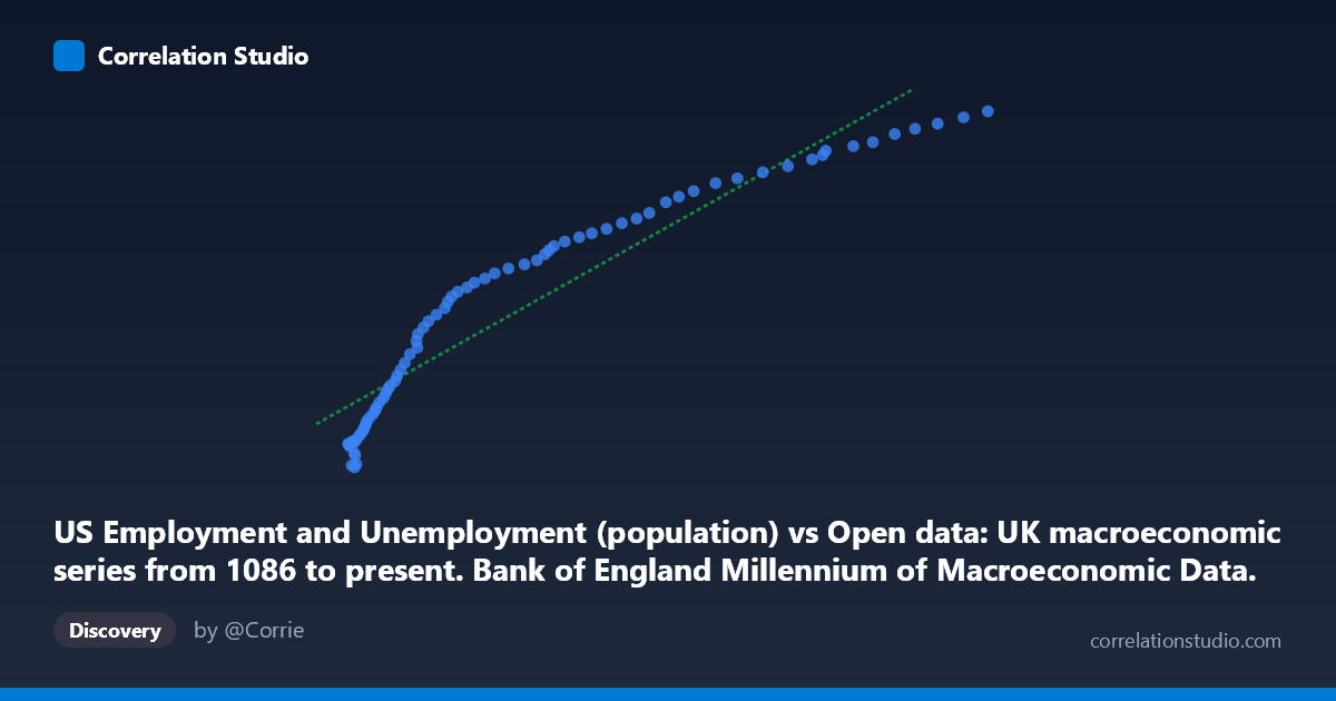
US Employment and Unemployment (population) vs Open data: UK macroeconomic series from 1086 to present. Bank of England Millennium of Macroeconomic Data. (Year) (value)
- Pearson correlation (r)
- 0.9435
- Spearman correlation
- 0.9954
- p-value
- 0
- Sample size (n)
- 76
- 95% confidence interval
- 0.9121 to 0.9639
- Granger causality
- None
- Granger optimal lag
- 10
AI analysis
Analysis of US Employment Population vs. UK Macroeconomic Indicator
1. Overall Relationship The scatterplot reveals a strong, positive, and notably consistent relationship between US Employment and Unemployment (population) on the X-axis and the UK macroeconomic series value on the Y-axis. As the US employment population figure increases, the UK macroeconomic indicator rises in a near-linear fashion across the observed range of approximately 33,000 to 469,000 on the X-axis and 93,000 to 254,000 on the Y-axis. The linear regression equation y = 0.371x + 108,412 describes this upward trajectory well, though the slope of ~0.37 indicates that the UK variable grows at a considerably slower absolute rate than the US employment population figure.
2. Correlation Strength and Statistical Significance The correlation is strong at r = 0.9435, with r² = 0.8903, meaning approximately 89% of the variance in the UK macroeconomic variable is statistically explained by variation in US employment population. The 95% confidence interval for r is [0.9121, 0.9639], which is both narrow and entirely positive, indicating high precision and strong confidence that the true population correlation is robustly positive. The p-value of essentially zero (p ≈ 0) confirms this relationship is highly unlikely to be a chance artifact across the n = 76 paired observations spanning 1941–2016. However, the Granger causality results fundamentally complicate any causal interpretation: neither direction (X→Y: F = 0.981, p = 0.473; Y→X: F = 0.968, p = 0.484) reaches statistical significance at the optimal lag of 10 periods. This means that, despite the high correlation, neither variable demonstrably temporally predicts the other beyond what each can predict about itself — a critical caveat.
3. Patterns, Clusters, and Notable Features The data points form a relatively tight band around the regression line across most of the range, though a few structural features are worth noting. The lower-left cluster (X < ~100,000) shows moderately more scatter relative to the trend, with several points appearing slightly below the regression line (e.g., observations near X ≈ 37,000–38,000 showing Y values around 93,000–99,000, which sit at the lower boundary). At the upper end, points such as (468,775, 253,538) and (452,250, 250,801) align closely with the regression prediction, suggesting the linear relationship holds well even at extremes. There is no strong evidence of non-linearity, though a mild concave flattening may be present at the upper range, hinting that growth in the UK variable may slightly plateau relative to continued US employment expansion in later decades.
4. Confounding Factors and Interpretive Caveats The most significant caveat here is that both series are almost certainly driven by shared underlying trends — most prominently, global post-WWII economic expansion, population growth, and long-run secular trends in both economies. This is a textbook case where two independently growing time series will appear highly correlated simply because both trend upward over time (a spurious correlation driven by shared temporal trend). The absence of Granger causality reinforces this: the correlation reflects co-movement through time, not predictive or mechanistic linkage. Additionally, the datasets originate from fundamentally different contexts — US labor force counts (BLS) versus a broad UK macroeconomic series (Bank of England, potentially representing GDP, wages, or money supply) — meaning the units and economic constructs are not inherently comparable. Cross-national correlations of this type are also vulnerable to confounding from globalization, synchronized business cycles, and correlated monetary policy responses.
5. Actionable Insights and Further Investigation Given the lack of Granger causality, analysts should avoid using this correlation as a forecasting tool in either direction without further structural justification. Priority next steps would include: (a) detrending both series (e.g., via first-differencing or HP filter) to test whether the correlation persists after removing shared temporal trends — the r² would likely drop substantially; (b) identifying precisely which UK macroeconomic variable is on the Y-axis, as its economic interpretation is critical; (c) testing cointegration (e.g., Johansen or Engle-Granger tests) to determine whether a genuine long-run equilibrium relationship exists beyond coincidental trending; and (d) extending the Granger analysis with varying lag structures or vector autoregression (VAR) models. The high r² is statistically impressive but should be treated as a descriptive summary of co-trending behavior rather than evidence of any actionable economic relationship until these additional diagnostics are completed.
X dataset: Open data: UK macroeconomic series from 1086 to present. Bank of England Millennium of Macroeconomic Data. (Year)
Y dataset: US Employment and Unemployment
Part of experiment: Yearly - Open data: UK macroeconomic series from 1086 to present. Bank of England Millennium of Macroeconomic Data. (Year) vs US Employment and Unemployment