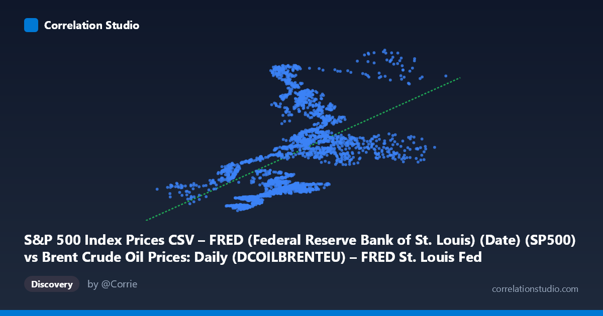
S&P 500 Index Prices CSV – FRED (Federal Reserve Bank of St. Louis) (Date) (SP500) vs Brent Crude Oil Prices: Daily (DCOILBRENTEU) – FRED St. Louis Fed (DCOILBRENTEU)
- Pearson correlation (r)
- 0.4795
- Spearman correlation
- 0.5862
- p-value
- 0
- Sample size (n)
- 2475
- 95% confidence interval
- 0.4485 to 0.5093
- Granger causality
- None
- Granger optimal lag
- 9
AI analysis
Analysis: Brent Crude Oil Prices vs. S&P 500 Index (2016–2026)
1. Overall Relationship Revealed
The scatterplot reveals a moderate positive relationship between daily Brent crude oil prices (X-axis) and S&P 500 index values (Y-axis) over approximately a decade of daily observations. As crude oil prices rise, S&P 500 values tend to trend higher as well, consistent with both variables responding to shared macroeconomic tailwinds — periods of strong global demand, economic expansion, and risk-on investor sentiment. However, the scatter is visibly wide, with considerable vertical dispersion at nearly every oil price level, making clear that oil prices alone are far from a reliable predictor of equity valuations. The linear regression line (y = 34.87x + 1,515.34) captures a positive slope, but the cloud of points around it suggests substantial unexplained variation throughout the full range.
2. Correlation Strength, Direction, and Temporal Causality
The Pearson correlation of r = 0.4795 indicates a moderate positive association, but the explanatory power is notably limited: r² = 0.2299 means only ~23% of variance in S&P 500 values is explained by Brent crude prices, leaving roughly 77% attributable to other factors entirely. The 95% confidence interval of [0.4485, 0.5093] is relatively tight given the large sample (n = 2,475), and the p-value of effectively zero confirms this correlation is statistically robust — not a sampling artifact. That said, statistical significance at this scale should not be conflated with practical or predictive significance. Critically, the Granger causality tests return no significant directional relationship in either direction (X→Y: F = 1.56, p = 0.12; Y→X: F = 0.97, p = 0.46), meaning neither variable meaningfully predicts the other's future values at the optimal 9-period lag. The correlation, while real, appears to reflect contemporaneous co-movement driven by shared external forces rather than any lead-lag predictive dynamic.
3. Notable Patterns, Clusters, and Non-Linear Features
Several structural features stand out in the sample points and overall distribution. There is a noticeable clustering of observations in the oil price range of roughly $45–$90/barrel, which corresponds to the bulk of the dataset's timeframe and reflects the post-2016 oil price regime. Within this dense central cluster, vertical scatter in S&P 500 values spans roughly 2,000 to 6,500+ points — an enormous range for a single X-band, underscoring the weak local predictive power. At higher oil prices (above ~$100), observations become sparser but show mixed S&P 500 outcomes, with some high-equity/high-oil combinations visible (e.g., ~$119 oil, ~6,825 S&P) alongside moderate equity values at similar oil levels. Importantly, the Spearman ρ exceeds Pearson r, which is a meaningful diagnostic flag suggesting the true relationship follows a monotonic but non-linear pattern — a logarithmic or polynomial fit would likely explain more variance than the linear model and reduce residual heteroscedasticity. Several apparent outliers with very high S&P values (6,000) at mid-range oil prices (~$67–$78) likely correspond to the 2024–2025 equity rally period.
4. Confounding Factors and Interpretive Caveats
This correlation is almost certainly spuriously inflated by shared exposure to a common driver: global macroeconomic conditions. Both asset classes tend to rise during periods of synchronized global growth and fall during recessions or demand shocks — making it difficult to isolate a direct causal mechanism. Several specific confounders deserve attention. First, Federal Reserve monetary policy profoundly influences both equity valuations (via discount rates) and commodity demand expectations simultaneously. Second, the COVID-19 period introduced extreme structural breaks — oil briefly went negative in April 2020 while equities crashed then rapidly recovered — creating unusual data points that could distort regression coefficients. Third, the USD exchange rate affects Brent crude pricing directly (it's dollar-denominated) while also influencing multinational earnings embedded in the S&P 500. Finally, the 10-year rolling window from FRED means the dataset spans markedly different regimes (low-rate expansion, pandemic shock, high-inflation tightening cycle), and treating this as a homogeneous population may obscure regime-specific relationships that run in opposite directions.
5. Actionable Insights and Further Investigation
Given the non-linear signal flagged by the Spearman/Pearson discrepancy, the most immediate analytical step would be to fit and compare logarithmic and polynomial regression models against the current linear specification — this could meaningfully improve explained variance beyond the current 23% baseline. Regime-segmented analysis (e.g., pre-COVID, COVID shock, post-COVID tightening, 2024–2026) would likely reveal that the correlation is highly unstable across time periods, which itself is strategically informative for risk management. From a practical standpoint, investors or analysts should resist using crude oil prices as a standalone equity market signal given the absence of Granger causality and the large unexplained variance. A more productive framing would be to investigate both variables as joint outputs of a latent global demand factor, potentially using principal component analysis or a structural VAR model with additional covariates (VIX, DXY, global PMI, Fed funds rate) to properly decompose their shared and idiosyncratic variance. Finally, rolling-window correlation analysis across the 10-year span would reveal whether the relationship has strengthened, weakened, or periodically reversed — a critical check before drawing any forward-looking inference.
X dataset: Brent Crude Oil Prices: Daily (DCOILBRENTEU) – FRED St. Louis Fed
Y dataset: S&P 500 Index Prices CSV – FRED (Federal Reserve Bank of St. Louis) (Date)
Part of experiment: Daily - Brent Crude Oil Prices: Daily (DCOILBRENTEU) – FRED St. Louis Fed vs S&P 500 Index Prices CSV – FRED (Federal Reserve Bank of St. Louis) (Date)