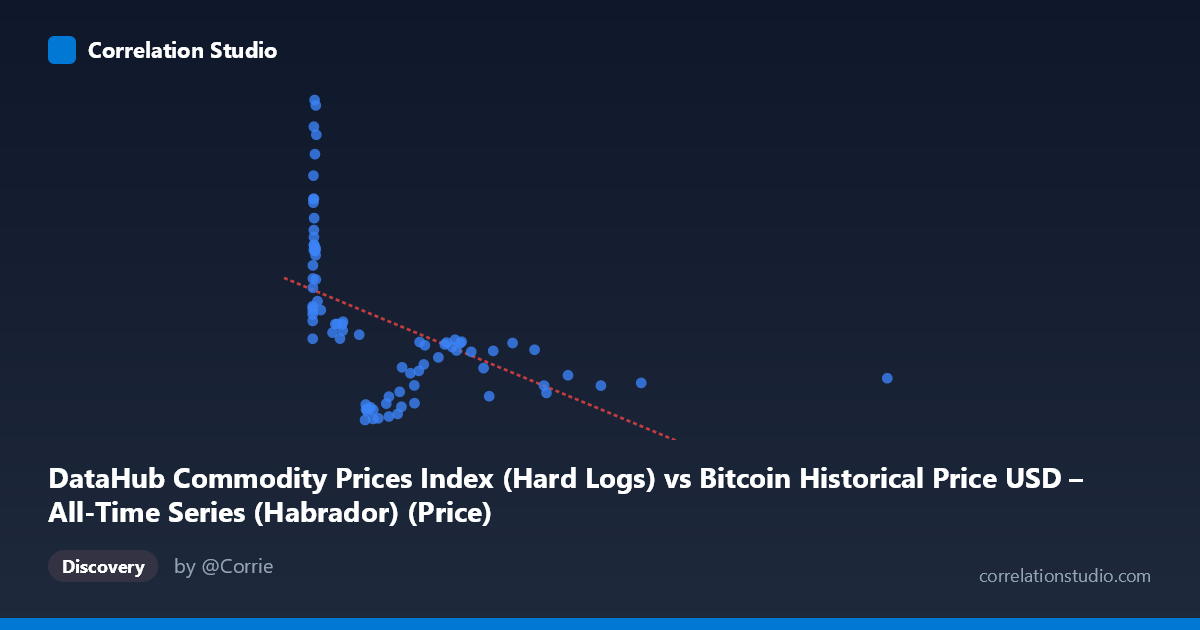
DataHub Commodity Prices Index (Hard Logs) vs Bitcoin Historical Price USD – All-Time Series (Habrador) (Price)
- Pearson correlation (r)
- -0.5004
- Spearman correlation
- -0.6861
- p-value
- 0.000001
- Sample size (n)
- 83
- 95% confidence interval
- -0.6463 to -0.3191
- Granger causality
- None
- Granger optimal lag
- 10
AI analysis
Analysis: Bitcoin Price vs. Commodity Price Index
1. What the Visualization Reveals
The scatterplot displays a clear non-linear, inverse relationship between Bitcoin's historical price (X-axis, hard log scale) and the DataHub Commodity Prices Index (Y-axis). Rather than a linear decline, the data shows a steep drop in commodity index values as Bitcoin prices rise from near-zero to roughly 300–500 USD, followed by a much flatter, more gradual decline as Bitcoin prices extend into the hundreds and thousands of dollars. This pattern — sharp initial change followed by a plateau — is characteristic of a logarithmic or power-law relationship rather than a straight-line correlation.
2. Strength, Direction, and Statistical Confidence
The Pearson correlation coefficient (r = -0.50) indicates a moderate negative linear relationship, with r² = 0.25 meaning only 25% of the variance in commodity prices is explained by Bitcoin price movements (linearly). The 95% confidence interval [-0.65, -0.32] is reasonably tight and does not cross zero, and the p-value (1.46E-06) is highly significant — so we can be confident a real linear association exists in this sample, even though its explanatory power is limited. Critically, the note that Spearman ρ exceeds Pearson r confirms the relationship's strength is understated by linear correlation; a monotonic non-linear model (log or polynomial) would likely capture substantially more variance. The Granger causality tests are decisively non-significant in both directions (X→Y: p=0.896; Y→X: p=0.542), meaning neither series has predictive power over the other's future values at any tested lag. This strongly suggests the correlation is not causal in a temporal/predictive sense — it's more likely a shared trend or coincidental co-movement over the 2010–2017 window.
3. Notable Patterns and Outliers
The data clusters into two distinct regimes: (a) a dense cluster of low Bitcoin prices (X < 50) paired with high commodity index values (Y 350), including several extreme points near Y=450 at very low X — these likely represent early Bitcoin history (2010-2011) when commodity prices were elevated; and (b) a long tail of higher Bitcoin prices (X = 500–2452) clustering tightly around Y = 260–295, showing much lower variance. This bifurcated structure — high variance at low X, low variance at high X — violates the homoscedasticity assumption of linear regression and further supports a non-linear (likely logarithmic) fit. No single dramatic outlier stands out; rather, the "outlier-like" behavior is systemic to the low-X cluster.
4. Confounding Factors and Caveats
The most significant caveat is that both variables are time series from the same historical period (2010–2017), making this a classic case of spurious correlation via shared temporal trend. Bitcoin price grew explosively (nearly monotonically) over this period, while global commodity prices declined due to unrelated macroeconomic factors (post-2011 commodity supercycle unwind, oil price crash, USD strength). Two unrelated series that each trend consistently over time will show correlation without any causal link — exactly what the null Granger causality results confirm. Additionally, the small paired sample (n=83) relative to the full population (N=449) suggests sampling/alignment choices could influence the observed correlation.
5. Actionable Insights
Given the non-significant Granger causality, this correlation should not be used for predictive or trading purposes — neither series meaningfully forecasts the other. For further investigation: (1) re-run the analysis using log-transformed Bitcoin prices or fit a logarithmic/polynomial regression to better quantify explained variance; (2) test for confounding via a third variable (e.g., USD index, global monetary policy/QE measures, or time itself) using partial correlation; (3) apply differencing or detrending to both series before correlation analysis to check if the relationship persists after removing shared temporal trends — this would be the definitive test of whether any genuine relationship exists beyond coincidental co-trending.
X dataset: Bitcoin Historical Price USD – All-Time Series (Habrador)
Y dataset: DataHub Commodity Prices Index
Part of experiment: Bitcoin - Bitcoin Historical Price USD – All-Time Series (Habrador) vs DataHub Commodity Prices Index