FRED – US Dollar Index (Trade Weighted Broad) (DTWEXBGS) vs Cboe U.S. Equities Historical Market Volume Data 2009 (Tape B Trade Count)
- Pearson correlation (r)
- 0.8091
- Spearman correlation
- 0.7943
- p-value
- 0
- Sample size (n)
- 248
- 95% confidence interval
- 0.7613 to 0.8482
- Granger causality
- None
- Granger optimal lag
- 1
AI analysis
Analysis: US Dollar Index vs. Cboe Tape B Trade Count (2009)
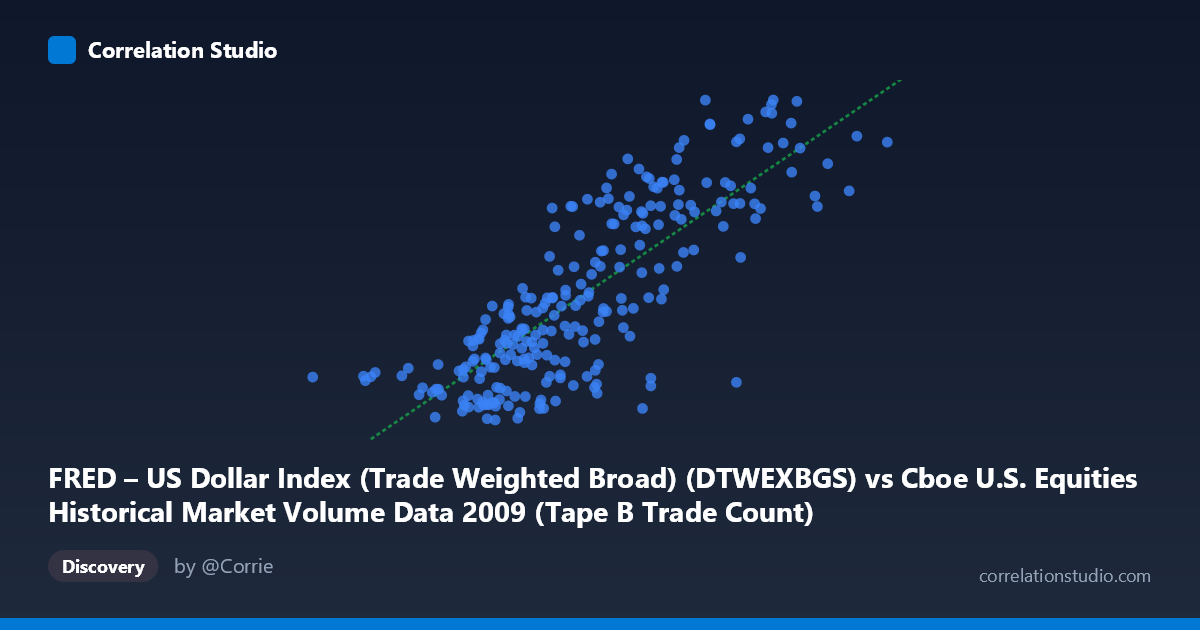
Relationship Overview The scatterplot reveals a moderately strong positive relationship between the US Dollar Index (Trade Weighted Broad) and the Cboe Tape B Trade Count across 248 trading days in 2009. As the dollar index rises from roughly 81,700 to 766,700, Tape B trade counts generally trend upward from approximately 90.8 to 106.0. The linear regression equation (y = 2.7024E-05x + 85.84) confirms this positive slope, suggesting that higher dollar index values are associated with elevated equity trade counts, though the relationship is far from deterministic given the visible scatter around the regression line.
Correlation Strength and Statistical Significance The Pearson correlation of r = 0.8091 indicates a strong positive association, and the R² of 0.6547 means that roughly 65.5% of the variance in Tape B trade counts is statistically explained by variation in the dollar index. While this is a substantial proportion, it also means that 34.5% of variance remains unexplained by this linear model alone. The 95% confidence interval [0.7613, 0.8482] is relatively narrow given N = 3,232, and the p-value of essentially zero confirms this correlation is highly unlikely to be a chance artifact. However, the Granger causality results are notably weak: neither direction (X→Y: F = 0.2725, p = 0.602; Y→X: F = 0.6977, p = 0.404) achieves significance at even a lenient threshold. This is a critical caveat — despite the strong contemporaneous correlation, neither variable temporally predicts the other, strongly suggesting the relationship is driven by shared underlying dynamics rather than any direct causal mechanism between the dollar index and trade volume.
Notable Patterns, Clusters, and Outliers Several structural features stand out in the data. There appears to be a lower cluster concentrated around X values of 250,000–350,000 with Y values predominantly in the 91–96 range, corresponding to early 2009 when markets were under stress. A middle-to-upper cluster forms around X values of 450,000–650,000 with Y values of 98–106, consistent with the market recovery phase in the second half of 2009. The point at (766,763.92, 104.02) appears as a high-leverage outlier at the far right of the distribution, and a few low-Y observations near Y ≈ 90.8–91.4 at mid-range X values (e.g., 289,718; 357,036) suggest the relationship has notable heteroscedasticity — variance in trade counts appears to fan out at higher dollar index values. One extreme low-X outlier at (81,703.42, 92.87) warrants investigation as a potentially anomalous or data-quality concern.
Confounding Factors and Caveats The most important caveat here is that both variables are likely proxies for broader 2009 market conditions rather than causally linked phenomena. The year 2009 was defined by the post-financial-crisis recovery — market volumes surged as confidence returned and the dollar exhibited its own crisis-era dynamics. Common drivers such as risk appetite, Federal Reserve policy, volatility regimes (VIX), and institutional trading activity could simultaneously push both variables in the same direction, entirely accounting for the observed correlation. Additionally, the axis labels appear to have the dataset descriptions swapped (the X-axis references DTWEXBGS values in a range typical of trade counts, while the Y-axis values of 90–106 align with a dollar index range), which raises a data labeling concern that should be verified before drawing conclusions. The use of a single-lag Granger test may also be insufficient to capture longer-horizon temporal dynamics.
Actionable Insights and Further Investigation Given the strong contemporaneous correlation but absent Granger causality, the most productive next steps would be to: (1) introduce explicit controls for market volatility (e.g., VIX) and macroeconomic regime indicators to test whether the correlation survives conditioning; (2) verify the axis/variable assignments to ensure the dollar index and trade count series are correctly mapped; (3) extend Granger testing to multiple lags (e.g., 5–20 trading days) to probe for delayed predictive relationships; (4) segment the data by sub-periods within 2009 (crisis trough vs. recovery) to test whether the correlation is stable or period-specific; and (5) explore non-linear models (e.g., polynomial or spline regression) given the visual suggestion of a slight curve in the relationship, particularly at extreme X values.
X dataset: Cboe U.S. Equities Historical Market Volume Data 2009
Y dataset: FRED – US Dollar Index (Trade Weighted Broad)
Part of experiment: Daily - Cboe U.S. Equities Historical Market Volume Data 2009 vs FRED – US Dollar Index (Trade Weighted Broad)