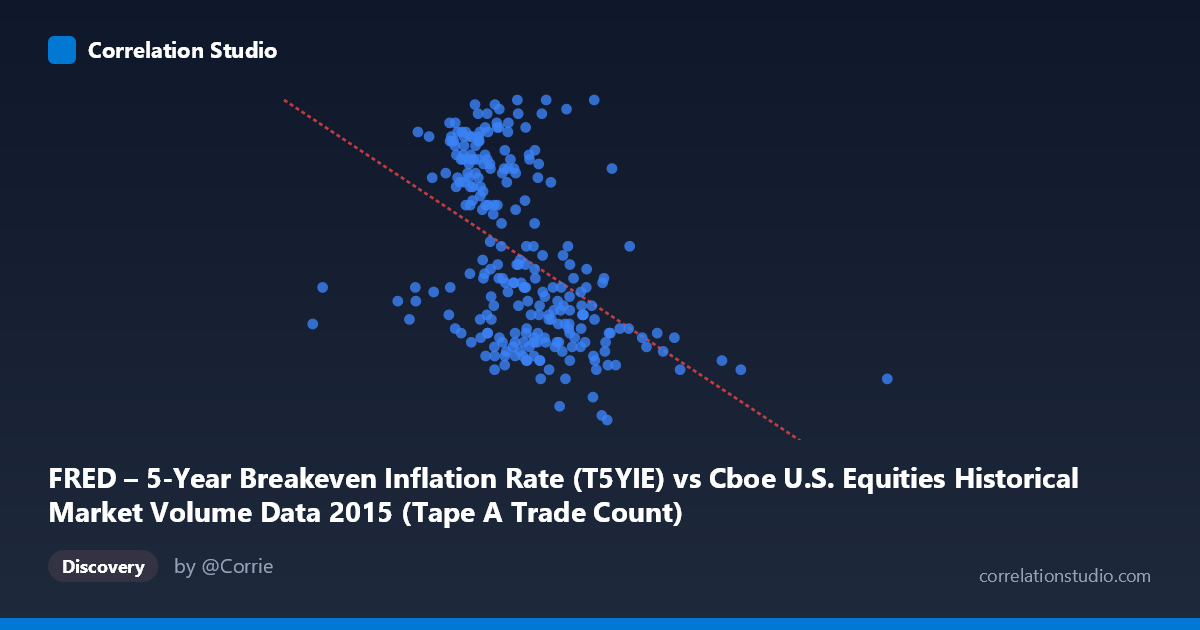
FRED – 5-Year Breakeven Inflation Rate (T5YIE) vs Cboe U.S. Equities Historical Market Volume Data 2015 (Tape A Trade Count)
- Pearson correlation (r)
- -0.4747
- Spearman correlation
- -0.5327
- p-value
- 0
- Sample size (n)
- 250
- 95% confidence interval
- -0.5655 to -0.3726
- Granger causality
- None
- Granger optimal lag
- 1
AI analysis
Analysis: 5-Year Breakeven Inflation Rate vs. Cboe Equity Trade Count (2015)
Relationship Overview The scatterplot reveals a moderate negative relationship between the FRED 5-Year Breakeven Inflation Rate (X-axis) and Cboe U.S. Equities Tape A Trade Count (Y-axis) across 2015 trading days. As breakeven inflation expectations rise, equity trade counts tend to decline, and conversely, lower inflation expectations coincide with higher trading activity. The linear regression equation (y = -3.53E-07x + 1.88) captures this downward slope, though considerable scatter around the regression line is immediately apparent, suggesting the relationship is real but far from deterministic. The data cloud spans a wide X-range (~576K to ~2.9M), with the bulk of observations clustering between roughly 1.1M and 1.9M on the X-axis and between 1.1 and 1.7 on the Y-axis.
Correlation Strength and Statistical Significance The Pearson correlation of r = -0.4747 indicates a moderate negative association. Critically, r² = 0.2253, meaning only about 22.5% of the variance in trade counts is explained by breakeven inflation rates — leaving roughly 77.5% attributable to other factors. The 95% confidence interval of [-0.5655, -0.3726] is meaningfully away from zero and reasonably tight, lending confidence that the negative direction is genuine. The p-value of 1.776E-15 is extraordinarily small against the N=3,302 population, confirming this is not a chance finding. However, the Granger causality results are notably null — neither direction (X→Y: F=0.071, p=0.790; Y→X: F=0.126, p=0.723) achieves significance at any conventional threshold. This is an important caveat: while a contemporaneous statistical correlation exists, neither variable temporally predicts the other at a one-period lag, undermining any simple causal narrative.
Patterns, Clusters, and Outliers Several structural features stand out in the data. There appears to be a dense central cluster around X ≈ 1.2M–1.5M and Y ≈ 1.1–1.7, consistent with the mean values (X̄ ≈ 1.43M, Ȳ ≈ 1.38). Notably, a handful of low-X outliers are visible at X < 700K (e.g., the points at ~576K and ~617K), which correspond to periods of very low breakeven inflation — potentially reflecting market stress episodes in early-to-mid 2015 when oil price declines suppressed inflation expectations. On the high-X end, a point near 2.9M stands out as an extreme outlier, likely representing a single anomalous trading day with unusually high volume. The vertical spread at any given X value is substantial, reinforcing that the relationship is probabilistic rather than structural. There is also a faint suggestion of non-linearity: trade counts appear relatively compressed at the high end of inflation expectations, possibly indicating a floor effect in trading activity.
Confounding Factors and Interpretive Caveats Several confounds complicate interpretation. First, both variables are time-indexed to 2015, meaning any shared temporal trend (e.g., a secular decline in breakeven inflation through 2015 due to falling oil prices coinciding with broader market volatility patterns) could be driving the apparent correlation as a spurious co-movement rather than a genuine economic link. Second, equity trade counts are influenced by VIX, earnings seasons, macro announcements, and index rebalancing — factors entirely independent of inflation expectations. Third, the axis labels appear to be swapped in the dataset metadata (FRED inflation data described under the Cboe column and vice versa), warranting careful verification of which series actually occupies which axis before drawing firm conclusions. Finally, the Granger causality null result at lag-1 strongly suggests that any relationship is contemporaneous and possibly driven by a common third factor such as macroeconomic uncertainty or Federal Reserve communications.
Actionable Insights and Further Investigation Given these findings, practitioners should treat this correlation as a signal worth investigating further rather than a trading rule. Recommended next steps include: (1) controlling for VIX and realized volatility in a multivariate regression to isolate the inflation expectation effect on volume; (2) testing longer Granger lags (e.g., 5–20 days) to check whether the predictive relationship emerges at longer horizons; (3) segmenting the data by market regime (e.g., pre/post Fed communication events in 2015) to determine whether the correlation is driven by specific episodes; and (4) resolving the potential axis/metadata mislabeling to ensure the analytical direction is correctly specified. The ~22.5% explained variance is non-trivial and suggests inflation expectations deserve inclusion as one component in a broader multi-factor equity market activity model, but should not be used in isolation.
X dataset: Cboe U.S. Equities Historical Market Volume Data 2015
Y dataset: FRED – 5-Year Breakeven Inflation Rate
Part of experiment: Daily - Cboe U.S. Equities Historical Market Volume Data 2015 vs FRED – 5-Year Breakeven Inflation Rate