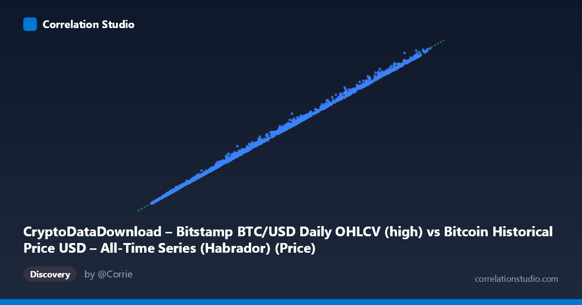
CryptoDataDownload – Bitstamp BTC/USD Daily OHLCV (high) vs Bitcoin Historical Price USD – All-Time Series (Habrador) (Price)
- Pearson correlation (r)
- 0.9997
- Spearman correlation
- 0.9998
- p-value
- 0
- Sample size (n)
- 4309
- 95% confidence interval
- 0.9997 to 0.9997
- Granger causality
- None
- Granger optimal lag
- 10
- Time coverage
- 2014-11-28 to 2026-09-15
- Recomputed on refreshed data
- 2026-10-24 (r was 0.9997)
AI analysis
Analysis: Bitcoin Price Series Cross-Reference (Habrador vs. Bitstamp OHLCV)
1. What the Visualization Reveals
The scatterplot shows an almost perfectly linear relationship between two Bitcoin price series spanning the same historical period (2014–2026), with values ranging from a few hundred dollars up to ~$125,000. Points hug a tight diagonal line across the entire range — from sub-$1,000 prices in the early years through the multi-thousand and eventually six-figure price levels of recent bull cycles. There is no visible curvature, fanning, or regime change; the relationship holds consistently across four orders of magnitude in price.
2. Strength, Direction, and Statistical Meaning
The correlation coefficient (r = 0.9997) and R² (0.9994) indicate that 99.94% of the variance in one series is explained by the other, with a regression slope near unity (1.0161) and a negligible intercept (~$118.5). This is about as strong a linear relationship as one can observe in real-world data. The 95% CI [0.9997, 0.9997] is essentially a point estimate — the sample size (n=4,170 daily observations) leaves virtually no uncertainty about the correlation's magnitude, and p≈0 confirms this is not a chance finding.
Critically, the Granger causality test shows no significant predictive direction in either direction (X→Y: p=0.547; Y→X: p=0.543). This is the expected and important finding: these are not two independent variables where one drives the other over time — they are two measurements of the same underlying asset price (Bitcoin/USD), recorded by different sources (a general historical dataset vs. Bitstamp's daily high). Neither "predicts" the other because they are contemporaneously reflecting the same market reality, not a lagged causal chain.
3. Notable Patterns and Outliers
While the overall fit is near-perfect, some sample points show meaningful divergence — e.g., (55027.46, 57737.00), (54458.04, 57402.89), (21310.66, 23777.00), and (5884.34, 6629.79), where Y exceeds X by 3–13%. These deviations likely correspond to periods of high volatility (rapid price swings within a day) where Bitstamp's daily "high" diverges more from whatever price point the Habrador dataset captures (e.g., close or a different snapshot time). This suggests the discrepancy is volatility-driven rather than random noise — larger absolute/percentage gaps tend to cluster in high-momentum price zones (e.g., past run-ups toward $20K, $55K).
4. Confounding Factors and Caveats
The near-perfect r² should not be mistaken for validation of two independent economic variables — it reflects data redundancy: both series describe the same asset's price history, likely sourced from overlapping exchange data or aggregation methods. Key caveats: - Differences in intraday timing (high vs. close vs. some blended metric) explain the minor residual scatter. - Exchange-specific price differences (Bitstamp vs. broader market aggregates) can create small but systematic gaps during volatile periods. - The heteroscedastic-looking absolute variance at high price levels is a scale artifact (percentage differences may be constant even as dollar differences grow).
5. Actionable Insights
- Use one series as a validation/QA check for the other rather than treating them as separate predictive signals — large deviations (like the ~5% gaps noted above) could flag data quality issues, missing timestamps, or exchange-specific anomalies worth auditing. - For any downstream modeling, only one series should be used to avoid multicollinearity — R²=0.9994 confirms these are effectively redundant. - Investigate whether residual deviations (X vs. Y) correlate with volatility (e.g., daily range or volume) — this could refine which series is preferable for high/low volatility regimes. - Confirm the exact field definitions (high vs. close, timezone/day boundaries) between the two datasets to fully explain the ~1.6% average residual slope offset from 1.0.
X dataset: Bitcoin Historical Price USD – All-Time Series (Habrador)
Y dataset: CryptoDataDownload – Bitstamp BTC/USD Daily OHLCV
Part of experiment: Bitcoin - Bitcoin Historical Price USD – All-Time Series (Habrador) vs CryptoDataDownload – Bitstamp BTC/USD Daily OHLCV