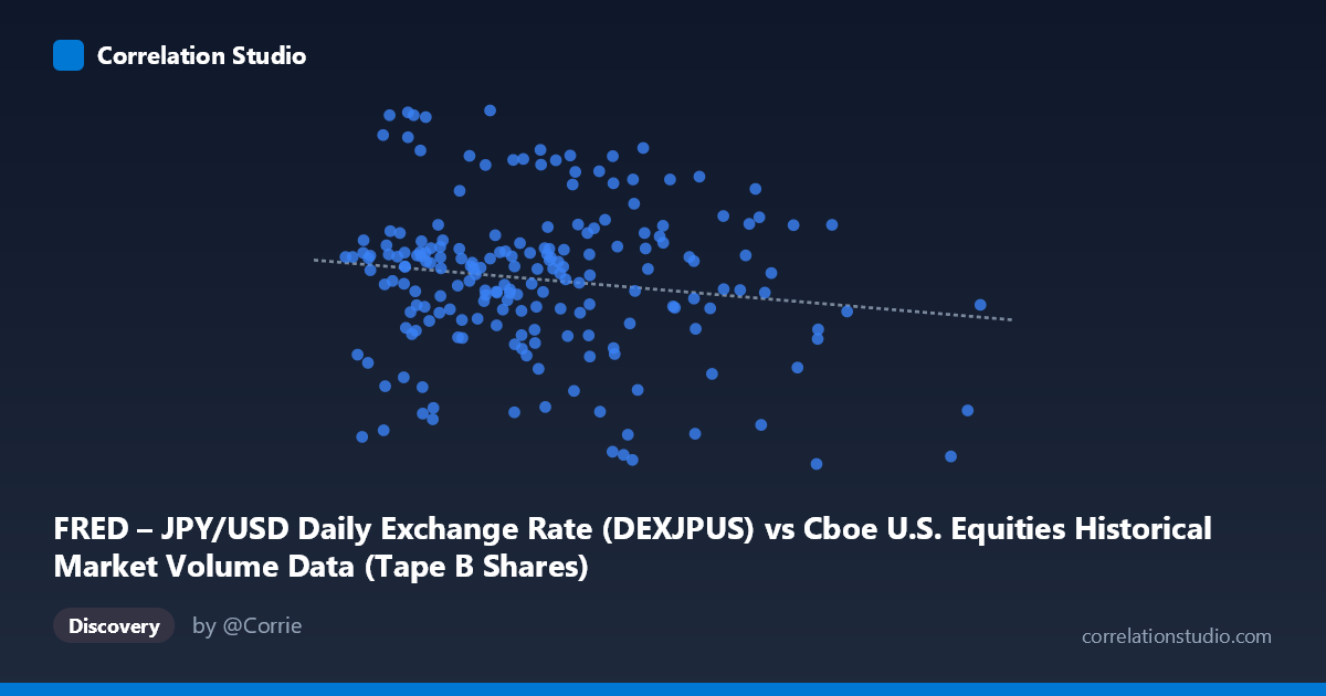
FRED – JPY/USD Daily Exchange Rate (DEXJPUS) vs Cboe U.S. Equities Historical Market Volume Data (Tape B Shares)
- Pearson correlation (r)
- -0.1463
- Spearman correlation
- -0.0638
- p-value
- 0.039725
- Sample size (n)
- 198
- 95% confidence interval
- -0.28 to -0.007
- Granger causality
- X → Y
- Granger optimal lag
- 1
- Time coverage
- 2026-01-02 to 2026-10-16
- Recomputed on refreshed data
- 2026-10-22 (r was -0.1463)
AI analysis
Scatterplot Analysis: JPY/USD Exchange Rate vs. Cboe Tape B Share Volume
Overall Relationship
The scatterplot reveals a moderate negative relationship between the JPY/USD daily exchange rate (X-axis, representing yen per dollar) and Cboe Tape B share volume (Y-axis). As the yen-per-dollar value increases — meaning the yen weakens relative to the dollar — Tape B share volumes tend to decline modestly. The linear regression equation (y = -1.46341E⁻⁰⁸x + 160.777) quantifies this: for every ~68 million unit increase in the JPY/USD rate, Tape B volume decreases by approximately 1 unit. Visually, the data cloud slopes gently downward from left to right, though with considerable scatter throughout, suggesting this is a real but noisy relationship rather than a tight mechanical one.
Correlation Strength and Statistical Significance
The Pearson correlation of r = -0.4158 indicates a moderate negative association. However, the coefficient of determination r² = 0.1729 is the more sobering figure — it means that only 17.3% of the variance in Tape B volume is explained by the JPY/USD rate, leaving roughly 82.7% attributable to other factors. The 95% confidence interval of [-0.5674, -0.2370] is entirely negative, confirming the direction is reliable, and the p-value of 2.06×10⁻⁵ is highly significant, making it extremely unlikely this correlation arose by chance given the sample of n = 98. That said, statistical significance here is partly a function of the broader population context (N = 1,980), and one should resist conflating significance with practical importance. Crucially, Granger causality tests show no significant predictive direction in either direction (X→Y: F = 0.666, p = 0.417; Y→X: F = 0.097, p = 0.756), meaning neither variable temporally predicts the other at a one-period lag — the correlation, while real, does not carry forecasting utility in a temporal sense.
Notable Patterns, Clusters, and Outliers
Several features stand out in the data. There is a visible cluster of lower-volume outliers at higher X values (roughly 300M–393M range), where Tape B volumes dip to the 152–155 range — points like (322,252,873; 152.64), (380,486,552; 152.88), and (393,280,831; 157.69) anchor the lower-right region. Conversely, at lower X values (136M–170M), volumes are predominantly elevated (158–160+), including the maximum at (158,227,178; 160.23). There also appears to be non-linear compression at very low X values, where volume approaches a ceiling near 160, suggesting possible saturation or a floor/ceiling effect in Tape B volume. The middle X range (190M–260M) shows the greatest vertical dispersion, spanning nearly the full Y range, which weakens the linear fit in that region considerably.
Confounding Factors and Interpretive Caveats
This correlation warrants considerable caution. The dataset labels appear internally inconsistent — the X-axis column is labeled as coming from Cboe volume data but represents the JPY/USD exchange rate, and vice versa for the Y-axis, suggesting a possible metadata mismatch that should be verified before drawing conclusions. Substantively, both series are likely driven by common macro factors — risk-on/risk-off market sentiment, Federal Reserve policy, and global equity volatility — making spurious correlation through shared confounders highly plausible. The time window (January–May 2026, ~98 trading days) is narrow, and seasonal patterns in equity volume (e.g., January effects, low summer volume) could interact with FX trends over this period. Additionally, Tape B specifically covers NYSE American and regional exchange stocks, which may have idiosyncratic volume drivers unrelated to currency dynamics.
Actionable Insights and Further Investigation
Given the lack of Granger causality, practitioners should not use JPY/USD movements to predict next-day Tape B volume or vice versa. However, the statistically significant contemporaneous correlation warrants further decomposition: researchers should test whether a latent third variable — such as the VIX, Fed funds rate expectations, or a broad risk appetite index — explains both series simultaneously. It would be valuable to extend the time series beyond five months to test whether this correlation is stable across different macro regimes. Researchers should also examine non-linear specifications (e.g., polynomial or piecewise regression) given the apparent ceiling effect at low X values. Finally, clarifying the data labeling discrepancy between dataset sources and axis assignments is a necessary first step before any further modeling or inference is pursued.
X dataset: Cboe U.S. Equities Historical Market Volume Data
Y dataset: FRED – JPY/USD Daily Exchange Rate
Part of experiment: Daily - Cboe U.S. Equities Historical Market Volume Data vs FRED – JPY/USD Daily Exchange Rate